Annex
A
(normative)
Mathematical foundations
This annex identifies the concepts from mathematics used in this International Standard and specifies the notation used for those concepts. No proofs are presented. A reader of this International Standard is assumed to be familiar with mathematics including set theory, linear algebra, and the calculus of several real variables as presented in reference works such as the Encyclopedic Dictionary of Mathematics [EDM].
An ordered set of n real numbers a where n is a natural number is
called an n-tuple of real numbers and shall be denoted by ![]() The
set of all n-tuples of real numbers is denoted by Rn. Rn is an n-dimensional vector space.
The
set of all n-tuples of real numbers is denoted by Rn. Rn is an n-dimensional vector space.
The canonical basis for Rn is defined as:
|
|
|
|
The elements of Rn may be called points or vectors. The latter term is used in the context of directions or vector space operations.
The zero vector ![]() is
denoted by 0.
is
denoted by 0.
Definitions A.2(a) through A.2(j) apply to any vectors![]() and
and ![]() in Rn:
in Rn:
a) The inner product or dot-product of two vectors x and y is defined as:
|
|
|
|
b)
Two vectors x
and y are called orthogonal if ![]() = 0.
= 0.
c) If n ≥ 2, two vectors x and y are called perpendicular if and only if they are orthogonal.
NOTE
1 If n ≥ 2, ![]() where
α is the angle between x
and y.
where
α is the angle between x
and y.
d) x is called orthogonal to a set of vectors if x is orthogonal to each vector that is a member of the set.
e) The norm of x is defined as
|
|
|
|
Note 2 The norm of x represents the length of the vector x. Only the zero vector 0 has norm zero.
f)
x is called normalized if![]() .
.
g) A set of two or more normalized and pair-wise orthogonal vectors is called an orthonormal set of vectors.
Example The canonical basis is an example of an orthonormal set of vectors.
h) The Euclidean metric d is defined by
|
|
d(x, y) = ||x – y||. |
|
i) The value of d(x, y) is called the Euclidean distance between x and y.
j) The cross product of two vectors x and y in R3 is defined as the vector:
|
|
|
|
Note 3 The vector x × y is orthogonal to both x and y, and
|
|
|
|
where α is the angle between vectors x and y.
A.3 The point set topology of Rn
Given a point p in Rn and a real value ε > 0, the set {q in Rn | d(p, q) < ε } is called the ε-neighbourhood of p.
Given a set D
 Rn and a point p, the
following terms are defined:
Rn and a point p, the
following terms are defined:
a) p is an interior point of D if at least one ε-neighbourhood of p is a subset of D.
b) The interior of a set D is the set of all points that are interior points of D.
NOTE 1 The interior of a set may be empty.
c) D is open if each point of D is an interior point of D. Consequently, D is open if it is equal to its interior.
d) p is a closure point of D if every ε-neighbourhood of p has a non-empty intersection with D.
Note 2 Every member of D is a closure point of D.
e) The closure of a set D is the set of all points that are closure points of D.
f) D is a closed set if it is equal to the closure set of D.
g) A set D is replete if all points in D belong to the closure of the interior of D.
Note 3 Every open set is replete. The union of an open set with any or all of its closure points forms a replete set. In particular, the closure of an open set is replete.
EXAMPLE 1 In R2 {(x, y) | -π < x < π, -π/2 < y < π/2} is open and therefore replete.
EXAMPLE 2 {(x, y) | -π < x ≤ π, -π/2 < y < π/2} is replete.
EXAMPLE 3 {(x, y) | -π ≤ x ≤ π, -π/2 ≤ y ≤ π/2} is closed and replete.
Many concepts traditionally defined on open sets can be extended by continuity to replete sets. In particular, if f is a continuous function defined on a replete set D, and if f is continuously differentiable on the interior of D, the derivative of f shall be extended by continuity to all of D.
NOTE 4 The usual definition of the derivative of a function is restricted to open sets.
A real-valued function f defined on a replete domain in Rn is called smooth if its first derivative exists and is continuous at each point in its domain.
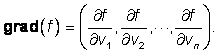
The gradient of f is the vector of first order partial derivatives
|
|
|
|
Definitions A.4(a) through A.4(g) apply to any vector-valued function F defined on a replete domain D in Rn with range in Rm
a)
The ith-component
function of a vector-valued function F is
the real-valued function fi defined by fi = ei •F
where ei is the
ith canonical basis vector, ![]() .
.
In this case:
|
|
F(v)
= (f1(v),
f2(v),
f3(v),
…, fn(v)) for v = (v1, v2, v3, …,vn) in D, |
|
b) F is called smooth if each component function fi is smooth, .
c) The first derivative of a smooth vector-valued function F, denoted dF, evaluated at a point in the domain is the n × m matrix of partial derivatives evaluated at the point:
|
|
|
|

d) The Jacobian matrix of F at the point v is the matrix of the first derivative of F.
NOTE 1 The rows of the Jacobian matrix are the gradients of the component functions of F.
e) In the case m = n, the Jacobian matrix is square and its determinant is called the Jacobian determinant.
f) In the case m = n, F is called orientation preserving if its Jacobian determinant is strictly positive for all points in D.
g) A vector-valued function F defined on Rn is linear if:
|
|
F(ax + y) = aF(x) + F(y) for all real scalars a and vectors x and y in Rn. |
|
NOTE 2 All linear functions are smooth.
A vector-valued function E
defined on Rn is affine if F, defined by![]() , is
a linear function. All affine functions on Rn are smooth.
, is
a linear function. All affine functions on Rn are smooth.
A function may be alternatively called an operator especially when attention is focused on how the function maps a set of points in its domain onto a corresponding set of points in its range.
EXAMPLE The localization operators (see 5.7)
If F
and G are two vector valued functions and the range of G is contained in the domain of F, then![]() , the composition of F with G, is the
function defined by
, the composition of F with G, is the
function defined by ![]()
![]() has the same domain as G,
and the range of
has the same domain as G,
and the range of ![]() is
contained in the range of F.
is
contained in the range of F.
Functional composition also applies to
scalar-valued functions f and g, If the range of g is contained
in the domain of f, then ![]() the composition of f with g, is the function defined by
the composition of f with g, is the function defined by ![]()
A.6.1 Implicit definition
A smooth surface in R3 is implicitly specified by a real-valued smooth function f defined on R3 as the set S of all points (x, y, z) in R3 satisfying:
a) f(x, y, z) = 0 and
b) grad( f )(x, y, z) ≠ 0.
In this case, f is called a surface generating function for the surface S.
EXAMPLE 1 If n ≠ 0 and p
are vectors in R3 and f(v) = n•(v – p), then f is smooth and ![]() The plane which is
perpendicular to n and contains p is the smooth surface
implicitly defined by the surface generating function f.
The plane which is
perpendicular to n and contains p is the smooth surface
implicitly defined by the surface generating function f.
Special cases:
When n = (1, 0, 0) and p = 0, the yz-plane is implicitly defined.
When n = (0, 1, 0) and p = 0, the xz-plane is implicitly defined.
When n = (0, 0, 1) and p = 0, the xy-plane is implicitly defined.
The surface normal n at a point p = (x, y, z) on the surface implicitly specified by a surface generating function f is defined as:
|
|
|
|

NOTE -n is also a surface normal to S at p. The surface generating function f determines the surface normal direction: n or -n.
The tangent plane to a surface at a point p = (x, y, z) on the surface S implicitly defined by a surface generating function f is the plane which is the smooth surface implicitly defined by h(v) = n • (v–p) where n is the surface normal to S at p.
EXAMPLE 2 If a and b are positive non-zero scalars, define
|
|
|
|
Then f is smooth and
|
|
|
|
is never (0, 0, 0) on the surface implicitly specified by the set satisfying f = 0.
A.6.2 Ellipsoid surfaces
If a and b are positive non-zero scalars, the smooth function:
|
|
|
|
is a surface generating function for a ellipsoid of revolution smooth surface S.
When b ≤ a, the surface is called an oblate ellipsoid. In this case a is called the major semi-axis29 of the oblate ellipsoid and b is called the minor semi-axis of the oblate ellipsoid.
The flattening of an oblate ellipsoid is defined as f = (a - b)/a.
The eccentricity of an oblate ellipsoid is defined as ![]() .
.
The second
eccentricity of an oblate ellipsoid is defined as ![]() .
.
When b = a, the oblate ellipsoid may be called a sphere of radius r = b = a.
When a < b, the surface is called a prolate ellipsoid. In this case, a is called the minor semi-axis of the prolate ellipsoid and b is called the major semi-axis of the prolate ellipsoid.
NOTE
1 A sphere of radius r is also implicitly
defined by the surface generating function ![]()
NOTE 2 The term spheroid is often used to denote an oblate ellipsoid with an eccentricity close to zero (“almost spherical”).
A smooth curve in Rn is parametrically specified by a smooth one-to-one Rn valued function F(t) defined on a replete interval I in R such that ||dF(t)|| ≠ 0 for any t in I.
EXAMPLE 1 If p and n are vectors in Rn such that n ≠ 0 and L(t) = p + t n, -∞ < t < +∞, then L is smooth and ||dL(t)|| = ||n|| > 0. The line which is parallel to n and which contains p is a smooth curve parametrically specified by L.
EXAMPLE 2 If a and b are positive non-zero scalars and b ≤ a, define
|
|
F(t) = (a cos(t), b sin(t)) for all t in the interval -p < t ≤ p. |
|
Then F is smooth and ||dF(t)|| ≥ b > 0 for all t in the interval and therefore parametrically specifies a smooth curve in R2.
An ellipse in R2 with major semi-axis a and minor semi-axis b, 0 < b ≤ a, is parametrically specified by:
|
|
F(t) = (a cos(t), b sin(t)), for all t in the interval -π < t ≤ π. |
|
A.7.1.2 Tangent to a smooth curve
If C(t) parametrically specifies a smooth curve C passing through a point p = C(tp), the tangent vector to C at p shall be defined as:
|
|
|
|
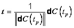
where dC(tp) = (dC1/dt, dC2/dt, …, dCn/dt) is the first derivative of C evaluated at tp.
NOTE -t is also a tangent vector to C at p. The parameterization function C(t) determines the tangent vector direction: t or -t.
A locus of points is a directed curve if it is the range of a smooth curve.
The tangent line to the curve C at p is a smooth curve parametrically specified by T(s) = p + s t, -∞ < s < +∞, where t is a tangent vector to C at p. See Figure A.1.
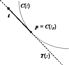
Figure A.1 — Tangent to a curve
If two parametrically specified smooth curves C1 and C2 intersect at a point p then the angle at p from C1 to C2 is defined as the angle from the tangent vector t1 to the tangent vector t2 of the two curves, respectively, at p. This is illustrated in Figure A.2.
Figure A.2 — Angle between two curves
A.7.1.4 Closed curve
If a smooth function F is defined on a closed and bounded interval I with interval end points t0 and t1 and if F parametrically specifies a smooth curve on the interior of I and p = F(t0) = F(t1), then F generates a closed curve through p.
EXAMPLE
|
|
F(t) = (a cos(t), b sin(t)), for all t in the interval -π+θ ≤ t ≤ π+θ. |
|
If a and b are positive non-zero scalars and θ is given, F generates a closed curve though p = (a cos(π+θ), b sin(π+θ))
A.7.1.5 Surface curves, connected and orientable surfaces
If C is a smooth curve in R3
parametrically specified by F on the
interval I and if S is a smooth surface generated by a surface generating function g, then C is a surface curve in S if ![]() for all t in I. In this case C shall be said to lie in
S.
for all t in I. In this case C shall be said to lie in
S.
EXAMPLE 1 If S is a smooth surface with generating function g and if C(s) defines a surface curve in S which passes through p = C(sp), then the tangent line to the curve at p, T(s) = p + s dC(tp), lies30 in the tangent plane to the surface S at p. This is illustrated in Figure A.3.

Figure A.3 — Tangent plane to a surface
A smooth surface S is connected if for any two distinct points in S, there exists a smooth surface curve parametrically specified by a smooth function defined on a bounded interval that lies in S and that contains the two points on the curve.
A connected surface S is called an orientable surface if the normal vector at an arbitrary point p on S can be continued in a unique and continuous manner to the entire surface. A normal vector at a fixed point p0 may be continued if there does not exist a closed curve C in S through p0 such that the normal vector direction reverses when it is displaced continuously from p0 along C and back to p0.
An oriented surface is an orientable surface in which one side has been designated as positive.
EXAMPLE 2 If S is implicitly defined by f = 0, the side bounding the set satisfying f > 0 is designated as the positive side.
EXAMPLE 3 A Möbius strip is an example of a non-orientable surface.
NOTE If S is implicitly specified, it is an orientable surface31.
A smooth curve in R2 may be implicitly specified by a real-valued smooth function f on R2 as the set S of all points (x, y) in R2 satisfying:
a) f(x, y) = 0 and
b) grad( f )(x, y) ≠ (0, 0).
In this case, f is called a curve generating function for the curve C.
EXAMPLE If a and b are positive non-zero scalars, define
|
|
|
|
Then f is smooth and
|
|
|
|
is never (0, 0) on the curve f = 0.
If 0 < b ≤ a, an ellipse in R2 with major semi-axis a and minor semi-axis b, is implicitly specified by the curve generating function defined by:
|
|
|
|
A.7.3 Arc length and geodesic distance
If p = F(tp) and q = F(tq) are two points on a smooth curve defined by F and tp < tq, the arc length from p to q along the curve is defined by
|
|
|
|
Given two distinct points p and q on a connected smooth surface S, a geodesic from p to q in S is a surface curve in S of minimal arc length that connects the two points. The geodesic distance from p to q in S is the arc length along a geodesic from p to q in S.
A.8 Special functions
A.8.1 Double argument arctangent function
The two argument form of inverse tangent, ![]() , returns a values adjusted by
the quadrant of the point
, returns a values adjusted by
the quadrant of the point ![]() .
Given real numbers
.
Given real numbers ![]()

NOTE If
![]() then
then ![]() Some software
implementation libraries reverse the roles of x and y.
Some software
implementation libraries reverse the roles of x and y.
A.8.2 Jacobian elliptic functions
Jacobian elliptic functions are defined in terms of certain elliptic integrals. There are many equivalent definitions, each involving special notation (see [ABST]). The notation used in this International Standard is given here.

the Jacobian elliptic functions used in this International Standard are defined by,
Series expansions for these Jacobian elliptic functions are given in [ABST].
NOTE The complex functions sn(w |ε2), cn(w |ε2) and dn(w |ε2) are called Jacobian elliptic functions in [ABST] and [DOZI] and are called Jacobi functions in [LLEE].
A.9 Projection function
A.9.1 Geometric projection functions into a developable surface
A projection function in R3 is a smooth function defined on a connected replete domain in R3 onto a surface in the domain whose points are all fixed points of the function. Projection functions defined below project their domain onto such a plane, cone, or cylinder surface and are classified as planar, conic, or cylindrical projection functions according to the class of the fixed-point surface.
NOTE Some map projections CSs are unrelated to any geometric projection.
A.9.2 Planar projection functions
A.9.2.1 Orthographic projection function
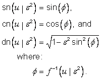
Given a plane in R3, the domain of the orthographic projection function is either all of R3 or the half space on one side of (and including) the plane. Given a point x in the domain, if x is not in the plane, there is one line that both passes through x and is perpendicular to the plane. If p is the point at the intersection of that line with the plane, the projection F assigns the value p to x. That is F(x) = p. If the point x lies in the plane, F(x) = x so that points in the plane are fixed points of the projection. In the case that the plane is the xy-plane, F(x, y, z) = (x, y, 0). See Figure A.4.
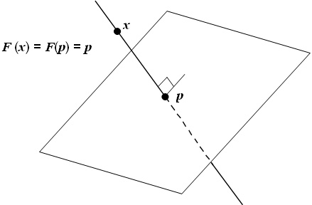
Figure A.4 — Orthographic projection
A.9.2.2 Perspective projection function
Given a plane in R3 and a point v (the vanishing point) not contained in the plane, the domain of the perspective projection function is the set of all points of R3 in the half space (including the plane) that does not contain the point v. Given a point x in the domain, there is one line that passes through both x and v. If p is the point at the intersection of the line with the plane, the projection F assigns the value p to x. That is F(x) = p. Note that if point q lies in the plane, F(q) = q so that it is a fixed point of the projection. See Figure A.5.
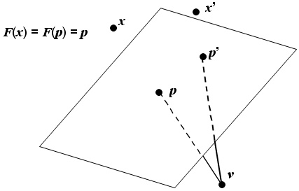
Figure A.5 — Perspective projection
A.9.2.3 Stereographic projection function
Given a plane in R3 and a point v not contained in the plane, the domain of the stereographic projection function is the set of all points of R3 in the half space on the point v side of (and including) the plane that are closer to the plane than the distance of v to the plane. Given a point x in the domain, there is one line that passes through both x and v. If p is the point at the intersection of the line with the plane, the projection F assigns the value p to x. That is F(x) = p. Note that if point q lies in the plane, F(q) = q so that it is a fixed point of the projection. See Figure A.6.
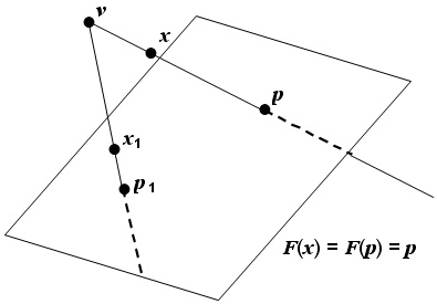
Figure A.6 — Stereographic projection
A.9.3 Cylindrical projection function
Given a cylinder and point v on its axis, a cylindrical projection function is defined on the domain R3 excluding the axis points as follows: Given a point x in the domain, there is one ray originating at v that passes through x. If p is the point at the intersection of the ray with the cylinder surface, the projection F assigns the value p to x. That is F(x) = p. Note that if point q lies on the cylinder surface, F(q) = q so that it is a fixed point of the projection. See Figure A.7.
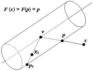
Figure A.7 — Cylindrical projection
A.9.4 Conic projection function
Given a (half) cone and point v on its axis inside the cone, a conic projection function projects a point x to the point p where p is the intersection of the cone with the ray from v through x. The domain of this projection is the union of all rays originating at v that intersects the cone and excluding the point v. See Figure A.8.
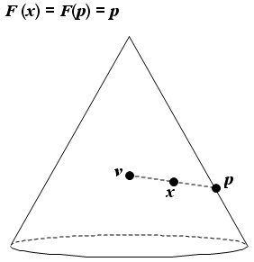
Figure A.8 — Conic projection