5 Abstract coordinate systems
5.1 Introduction
An abstract coordinate system is a means of identifying positions in position-space by coordinate n-tuples. An abstract coordinate system is completely defined in terms of the mathematical structure of position-space. In this International Standard the term “coordinate system”, if not otherwise qualified, is defined to mean “abstract coordinate system.” Each coordinate system has a coordinate system type (see 5.4). Other coordinate system related concepts defined in this clause include coordinate-component surfaces and coordinate-component curves (see 5.5), linearity and other properties (see 5.6), and localization (see 5.7). Map projections and augmented map projections are defined and treated as special cases of the general abstract coordinate system concept (see 5.8). Standardized abstract coordinate systems are specified in 5.9.
In Clause 6 a temporal coordinate system is defined as a means of identifying events in the time continuum by coordinate 1-tuples using an abstract coordinate system of coordinate system type 1D. In Clause 8 a spatial coordinate system is defined as an abstract coordinate system suitably combined with a normal embedding (see Clause 7) as a means of identifying points in object-space by coordinate n-tuples.
5.2 Preliminaries
This International Standard takes a functional approach to the construction of coordinate systems. Annex A provides a concise summary of mathematical concepts and specifies the notational conventions used in this International Standard. In particular, Annex A defines the terms interior, one-to-one, smooth, smooth surface, smooth curve, orientation-preserving, and connected. The concept of Rn as a vector space, the point-set topology of Rn, and the theory of real-valued functions on Rn are all assumed. Algebraic and analytic geometry, including the concepts of point, line, and plane, are also assumed. Together with such common concepts, a newly introduced concept replete will be used. A set D is replete if all points in D belong to the closure of the interior of D (see Annex A). A replete set is a generalization of an open set that allows the inclusion of boundary points. Boundary points are important in the definitions of certain coordinate systems.
5.3 Abstract CS
An abstract Coordinate System (CS) is a means of identifying a set of positions in an abstract Euclidean space that shall be comprised of:
a) a CS domain,
b) a generating function, and
c) a CS range,
where:
a) The CS domain shall be a connected replete domain in the Euclidean space of n-tuples (1 ≤ n ≤ m), called the coordinate-space.
b) The generating function shall be a one-to-one, smooth, orientation-preserving function from the CS domain onto the CS range.
c) The CS range shall be a set of positions in a Euclidean space of dimension m (n ≤ m ≤ 3), called the position-space. When n = 2 and m = 3, the CS range shall be a subset of a smooth surface5. When n = 1 and m = 2 or 3, the CS range shall be a subset of an implicitly specified smooth curve6.
An element of the CS domain shall be called a coordinate7. The kth-component of a coordinate n-tuple (1 ≤ k ≤ n) may be called the kth coordinate-component. Coordinate-component8 is the collective term for any kth coordinate-component.
An element of the CS range shall be called a position. The coordinate of a position p shall be the unique coordinate whose generating function value is p.
The generating function may be parameterized. The generating function parameters (if any) shall be called the CS parameters.
The inverse of the generating function shall be called the inverse generating function. The inverse generating function is one-to-one and is smooth and orientation-preserving in the interior of its domain. A CS may equivalently be defined by specifying the inverse generating function when the CS domain is an open set.
NOTE 1 The generating function of a CS is often specified by an algebraic and/or trigonometric description of a geometric relationship (see 5.3 Example). There are also CSs that do not have geometric derivations. The Mercator map projection (see Table 5.18) is specified to satisfy a functional requirement of conformality (see 5.8.3.2) rather than by a geometric construction.
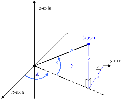
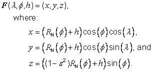
EXAMPLE Polar CS: Considering the polar geometry depicted in Figure 5.1, define a generating function F as:
![]()
where:
![]()
The CS domain of F in
coordinate-space is ![]() .
.
The CS range of F in
position-space is ![]() .
.
This generating function is illustrated in Figure 5.2. The grey boxes with lighter grey edges in this figure represent the fact that the range in position-space extends indefinitely, and that the domain in coordinate-space extends indefinitely along the r-axis. The dotted grey edges indicate an open boundary. This CS range, CS domain, and generating function define an abstract CS representing polar coordinates as defined in mathematics [EDM, “Coordinates”]. The normative definition of the polar CS may be found in Table 5.33.
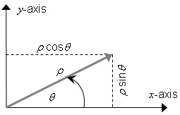
Figure 5.1 — Polar CS geometry
Figure 5.2 — The polar CS generating function
NOTE 2 In the special case where 1) the CS domain and CS range are both Rn and 2) the function is the identity function, this approach to defining coordinate systems reduces to the usual definition of the Euclidean coordinate system on Rn where each point is identified by an n-tuple of real numbers [EDM] (see Table 5.8, Table 5.29 and Table 5.35).
NOTE 3 The CS generating function has an inverse because it is one-to-one, but the inverse may be discontinuous at points in the image of CS domain boundary points. This is the case for the positive x-axis in the example above.
5.4 CS types
The coordinate-space and position-space dimensions characterize an abstract CS by CS type as defined in Table 5.1.
|
CS type |
Dimension of coordinate-space |
Dimension of position-space |
|
3D |
3 |
3 |
|
surface |
2 |
3 |
|
curve9 |
1 |
3 |
|
2D |
2 |
2 |
|
plane curve9 |
1 |
2 |
|
1D |
1 |
1 |
A CS of CS type 3D may be called a 3D CS, a CS of CS type surface may be called a surface CS, and a CS of CS type 2D may be called a 2D CS.
5.5 Coordinate surfaces, induced surface CSs, and coordinate curves
5.5.1 Introduction
The generating function of a 3D CS is a function of the three coordinate-components of a coordinate 3-tuple. If one of the coordinate-components is held fixed (to a constant value), then the generating function thus restricted to two variables may be viewed as a surface CS generating function (with a surface CS range). If two of the three coordinate-components are held fixed, the generating function restricted to one variable may be viewed as a curve CS generating function (with curve CS range). These observations motivate the definitions of coordinate-component surfaces and curves. The coordinate-component surface and coordinate-component curve concepts are required to specify induced CS relationships, for the definition of special coordinate curves parallel and meridian, and the definition of CS handedness (see also 10.5).
5.5.2 Coordinate-component surfaces and induced surface CSs
If F is the generating function of a 3D CS, and u = (u0, v0, w0) is in the interior of the CS domain D, then three surface CS generating functions at u are defined by:
![]() ,
,
![]() , and
, and
![]() .
.
The CS domain for S1 is the connected component of ![]() which contains (v0, w0).
which contains (v0, w0).
The CS domain for S2 is the connected component of ![]() which contains (u0, w0).
which contains (u0, w0).
The CS domain for S3 is the connected component of ![]() which contains (u0, v0).
which contains (u0, v0).
Each of these surface CSs shall be called, respectively, the 1st, 2nd, and 3rd surface CS induced by F at u.
The CS ranges of these surface CSs are, respectively, the 1st, 2nd, and 3rd coordinate-component surface at u.
EXAMPLE 1 Coordinate-component
surface: The geodetic 3D CS with generating function ![]() is specified in Table 5.14 with CS parameters a and b. The 3rd coordinate-component surface at
is specified in Table 5.14 with CS parameters a and b. The 3rd coordinate-component surface at ![]() is the surface of the
oblate ellipsoid with major semi-axis a and minor semi-axis b.
is the surface of the
oblate ellipsoid with major semi-axis a and minor semi-axis b.
EXAMPLE 2 Induced
surface CS: The surface geodetic CS is specified in Table 5.24. Its CS domain, CS range and
generating function are identical to the 3rd surface CS induced by
the geodetic 3D generating function at ![]() . If h is replaced by 0 in the
formulae for the generating and inverse generating functions of the geodetic 3D
CS, they reduce to the surface geodetic formulae.
. If h is replaced by 0 in the
formulae for the generating and inverse generating functions of the geodetic 3D
CS, they reduce to the surface geodetic formulae.
5.5.3 Coordinate-component curves
Coordinate-component curves are defined for CSs of CS type 3D, CS type surface, and CS type 2D.
The CS type 3D case:
If F is the generating function of a CS of CS type 3D, D is the CS domain, and u = (u0, v0, w0) is in the interior of D, then the 1st, 2nd, and 3rd coordinate-component curves at u are parametrically specified, respectively, by the following smooth functions:
![]() ,
,
![]() , and
, and
![]() .
.
The domain for C1 is the connected component of ![]() which contains u0.
which contains u0.
The domain for C2 is the connected component of ![]() which contains v0.
which contains v0.
The domain for C3 is the connected component of ![]() which contains w0.
which contains w0.
NOTE The
intersection of two coordinate surfaces at u is
(the locus of) a coordinate-component curve: ![]()
The CS type surface and CS type 2D cases:
If F is the generating function of a CS of CS type surface or CS type 2D, D is the CS domain, and u = (u0, v0) is in the interior of D, then the 1st and 2nd coordinate-component curve at u is parametrically specified, respectively, by the following smooth functions:
![]() , and
, and
![]() .
.
The domain for C1 is the connected component of ![]() which contains u0.
which contains u0.
The domain for C2 is the connected component of ![]() which contains v0.
which contains v0.
EXAMPLE If
![]() is in the interior of
the CS domain of the polar CS generating function F of the 5.3 Example, then the first
coordinate-component curve is
is in the interior of
the CS domain of the polar CS generating function F of the 5.3 Example, then the first
coordinate-component curve is![]() ,
and the 2nd coordinate-component curve is
,
and the 2nd coordinate-component curve is![]() .
.
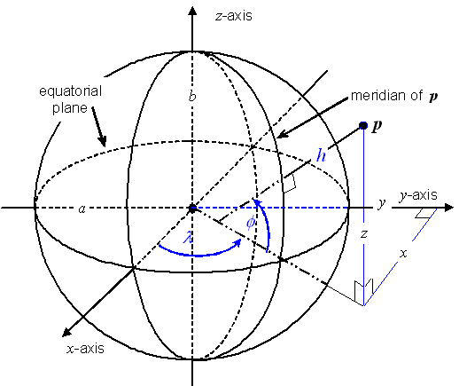
If F is the generating function for the geodetic 3D CS or the surface
geodetic CS, and ![]() in
the 3D case or
in
the 3D case or ![]() in
the surface case, then (see Figure 5.3):
in
the surface case, then (see Figure 5.3):
a) the 1st coordinate-component curve at u shall be called the parallel at u, and
b) the 2nd coordinate-component curve at u shall be called the meridian10 at u.
The meridian at ![]() shall
be called the prime
meridian11.
shall
be called the prime
meridian11.
The parallel at ![]() shall
be called the equator.
shall
be called the equator.
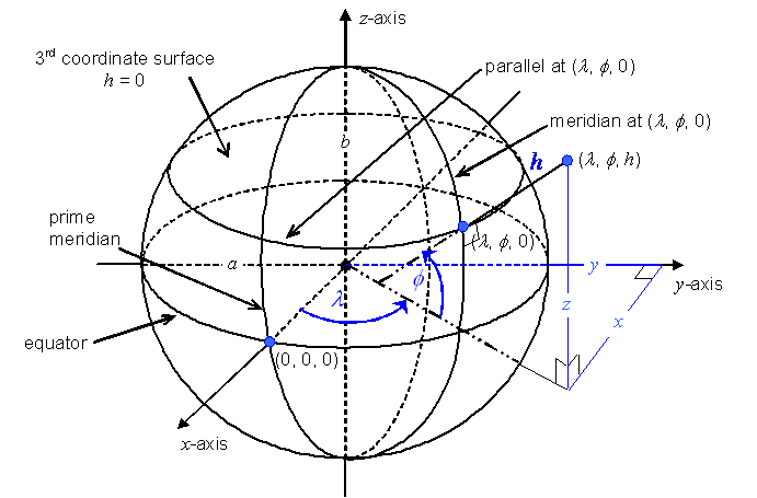
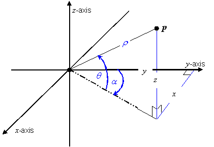
Figure 5.3 — Geodetic 3D CS geometry, and coordinate-component surface and curves
5.6 CS properties
5.6.1 Linearity
A CS with generating function F is
a linear CS if F is
an affine function. The CS domain of a linear coordinate system is all of the
coordinate-space![]() .
.
A curvilinear CS is a non-linear CS.
EXAMPLE The polar CS of 5.3 EXAMPLE is a curvilinear CS of CS type 2D.
5.6.2 Orthogonality
A CS of CS type 3D, CS type surface, or CS type 2D is orthogonal if the angle between any two coordinate-component curves at u is a right angle when u is any coordinate in the interior of the CS domain of the generating function.
EXAMPLE The polar CS of 5.3 EXAMPLE is a orthogonal CS of CS type 2D.
5.6.3 Linear CS properties: Cartesian, and orthonormal
In a linear CS, the kth coordinate-component curve is a line. The kth coordinate-component curve at the origin 0 of a linear CS is the kth-axis.
In a linear CS, if the angles between coordinate-component curves at the origin 0 are (pair-wise) right angles, then that is the case at all points. In particular, a linear CS is orthogonal12 if the axes are orthogonal.
In some publications a Cartesian CS is defined the same way as an
orthogonal linear CS13. This International Standard, however, defines this concept
differently. A linear CS with generating function F is
a Cartesian CS if ![]() (i.e., the axis unit points are all one
unit distant from the origin F(0)).
(i.e., the axis unit points are all one
unit distant from the origin F(0)).
An orthonormal CS is a linear CS that is both orthogonal and Cartesian.
A CS of CS type 3D with generating function F is orientation-preserving if the Jacobian determinant of F is positive.
EXAMPLE The Lococentric Euclidean 3D CS specified in Table 5.9 is an orientation-preserving orthonormal CS.
5.6.4 CS right-handedness and coordinate-component ordering
Given a CS of CS type 3D and a coordinate ![]() in the interior of the CS domain, the coordinate-component curves
at p determine an ordered set of three tangent vectors:
in the interior of the CS domain, the coordinate-component curves
at p determine an ordered set of three tangent vectors:

An orthogonal CS of CS type 3D is a right-handed CS if for some coordinate ![]() in the interior of the CS domain, the ordered set of tangent
vectors t1, t2, and t3 form a right-handed coordinate
system as defined in IS0 31-11.
The right-handed CS property is determined, in part, by the order of the
coordinate-components in the coordinate 3-tuple. The order of the
coordinate-components in the specification of an orthogonal CS of CS type 3D shall
be restricted to an ordering that insures a right-handed CS. This restriction
is required for uniform treatment of directions in an SRF (see 10.5).
in the interior of the CS domain, the ordered set of tangent
vectors t1, t2, and t3 form a right-handed coordinate
system as defined in IS0 31-11.
The right-handed CS property is determined, in part, by the order of the
coordinate-components in the coordinate 3-tuple. The order of the
coordinate-components in the specification of an orthogonal CS of CS type 3D shall
be restricted to an ordering that insures a right-handed CS. This restriction
is required for uniform treatment of directions in an SRF (see 10.5).
The coordinate-component ordering in the specification of a surface CS that is induced on a coordinate-component surface of a 3D CS, shall use the coordinate-component order of the inducing 3D CS.
EXAMPLE 1 The geodetic 3D CS (Table 5.14)
coordinate-component ordering ![]() insures
that the CS is right-handed. A similar ordering for the planetodetic 3D CS (Table
5.15) is not right-handed because the tangent to planetodetic
longitude points opposite to the direction of the tangent to geodetic
longitude. Instead, the coordinate-component ordering
insures
that the CS is right-handed. A similar ordering for the planetodetic 3D CS (Table
5.15) is not right-handed because the tangent to planetodetic
longitude points opposite to the direction of the tangent to geodetic
longitude. Instead, the coordinate-component ordering ![]() is specified to
satisfy the right-handed CS requirement.
is specified to
satisfy the right-handed CS requirement.
EXAMPLE 2 The surface planetodetic geodetic CS (Table 5.25)) coordinate-component ordering ![]() is determined by the
coordinate-component ordering
is determined by the
coordinate-component ordering ![]() of
the planetodetic 3D CS (Table 5.15).
of
the planetodetic 3D CS (Table 5.15).
5.7 CS localization
In some applications of a CS in the context of a spatial reference frame, it is necessary to consider a modified version of the CS that has been translated to a local origin and/or rotated (see "Lococentric" spatial reference frame variants in Clause 8). To treat these modifications in a uniform manner, the generating function of a CS that has been translated to a local origin and/or rotated is related to the generating function of the original CS by means of a localization operator. This uniform method, defined below, of specifying the variant CS by composing the original CS generating function with a localization operator shall be called CS localization.
Three parameterized operators, called localization operators, that operate on or between position-spaces are defined in Table 5.2. The inverses of these operators are defined in Table 5.3.
Table 5.2 — Localization operators
|
Localization |
Domain |
Range |
Localization parameters |
Operator definition |
|
|
|
|
q, r,
s, in |
|
|
|
|
|
q, r,
s, in |
|
|
|
|
|
q, r,
s, in |
|

Table 5.3 — Localization inverse operators
|
Localization operator |
Inverse operator definition |
|
|
|
|
|
|
|
|
|
There are several forms of CS localization depending on CS type and
localization operator. A 3D or surface CS with generating function F is
localized by composing F with the ![]() localization
operator. The localized CS is of the same CS type (CS type 3D or CS type surface,
respectively). Its generating function is
localization
operator. The localized CS is of the same CS type (CS type 3D or CS type surface,
respectively). Its generating function is ![]() and has the same CS
domain as F.
and has the same CS
domain as F.
There are two localization operators for a 2D CS. One uses localization
parameters in ![]() and
produces a surface CS. The other uses localization parameters in
and
produces a surface CS. The other uses localization parameters in ![]() and produces a 2D
CS.
and produces a 2D
CS.
a.
A 2D CS with generating function FC is localized by composing F with the ![]() localization
operator. The localized CS is a surface CS. Its generating function is
localization
operator. The localized CS is a surface CS. Its generating function is ![]() and has the same CS
domain as F.
and has the same CS
domain as F.
b.
A 2D CS with generating function F is
localized by composing F with the ![]() localization
operator. The localized CS is a surface CS. Its generating function is
localization
operator. The localized CS is a surface CS. Its generating function is ![]() and has the same CS
domain as F.
and has the same CS
domain as F.
The localization operator parameter q shall be called the lococentre. A localized CS may be called a lococentric CS.
NOTE CS localization preserves the following CS properties: linear/curvilinear, orthogonal, Cartesian, and orthonormal.
The relationship between a CS type and its localized version(s) is summarized in Table 5.4.
Table 5.4 — Localized CS type relationships
|
CS type |
Localization operator |
Lococentric CS type |
|
3D |
|
3D |
|
Surface |
|
Surface |
|
2D |
|
|
|
|
2D |
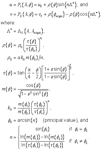
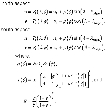
5.8 Map projection coordinate systems
5.8.1 Map projections
Map projections are 2D models of a 3D curved surface. In this International Standard, map projections are limited to the surface of an oblate ellipsoid. A map projection (MP) is comprised of
a) an MP domain in the surface of an oblate ellipsoid,
b) a generating projection, and
c) an MP range in 2D coordinate-space,
where:
a) the MP domain is a connected subset of the surface of the oblate ellipsoid,
b) the MP range is a connected replete set, and
c) the generating projection is one-to-one from the MP domain in the oblate ellipsoid onto its MP range and its inverse function is smooth and orientation-preserving in the MP range interior.
NOTE 1 This definition may be generalized to any ellipsoid including tri-axial ellipsoids, but this International Standard only addresses map projections for oblate ellipsoids.
NOTE 2 The domain of a map projection is always a proper subset of the oblate ellipsoid surface. In particular, the domain of the Mercator map projection (see Table 5.18) omits the pole points.
The generating projection P is
specified in terms of surface geodetic CS coordinates (see Table 5.24). The component functions ![]() and
and ![]() of the generating projection P
shall be called the mapping equations:
of the generating projection P
shall be called the mapping equations:
![]()
where:

The MP range coordinate-components u and v shall be called easting and northing, respectively. The positive direction of the u-axis (the easting axis) shall be called map-east. The positive direction of the v-axis (the northing axis) shall be called map-north.
The inverse mapping equations are the
component functions ![]() and
and
![]() of the inverse
generating projection
of the inverse
generating projection![]() :
:

5.8.2 Map projection as a surface CS
If the inverse generating projection of a map projection Q is
composed with the surface geodetic CS generating function![]() , the resulting
function
, the resulting
function ![]() is the
generating function of a surface CS (see Figure 5.4). The
CS domain is the MP range. In this International Standard, a map projection CS shall be a
surface CS for which the generating function is implicitly specified in terms
of the mapping equations of a map projection.
is the
generating function of a surface CS (see Figure 5.4). The
CS domain is the MP range. In this International Standard, a map projection CS shall be a
surface CS for which the generating function is implicitly specified in terms
of the mapping equations of a map projection.
In some cases, the surface geodetic coordinates with
coordinate-component ![]() are
not in the MP domain of P nor are they in the range of Q.
However, if the composite function
are
not in the MP domain of P nor are they in the range of Q.
However, if the composite function ![]() is
continuous at the pole points
is
continuous at the pole points![]() ,
then
,
then ![]() and
and ![]() shall be extended by
continuity to include the pole points in the CS range.
shall be extended by
continuity to include the pole points in the CS range.
NOTE The
CS generating function ![]() is
not to be confused with the generating projection P.
is
not to be confused with the generating projection P.
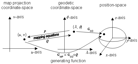
Figure 5.4 — The generating function of a map projection
5.8.3 Map projection geometry
5.8.3.1 Introduction
In general, the Euclidean geometry that a surface CS 2D
coordinate-space inherits from ![]() has
no direct significance with respect to the geometry of position-space. In
particular, the Euclidean distance between a pair of surface geodetic
coordinates has no obvious meaning in position-space. In contrast, map
projections are specifically designed so that coordinate-space geometry will
model one or more geometric aspects of the corresponding oblate ellipsoid
surface in position-space.
has
no direct significance with respect to the geometry of position-space. In
particular, the Euclidean distance between a pair of surface geodetic
coordinates has no obvious meaning in position-space. In contrast, map
projections are specifically designed so that coordinate-space geometry will
model one or more geometric aspects of the corresponding oblate ellipsoid
surface in position-space.
The map projection CSs specified in this International Standard are designed so that one or more geometric aspects of the MP domain in the oblate ellipsoid surface are approximated or modelled by the corresponding aspect in coordinate-space. The length of the line segment between two map coordinates is related to the length of the corresponding surface curve. Similarly, one or more of directions, areas, the angles between two intersecting curves, and shapes may be related approximately or exactly to the corresponding geometric aspect on the oblate ellipsoid surface.
The extent to which these aspects are or are not closely related is an indication of distortion. Some map projection CSs are designed to eliminate distortion for one geometric aspect (such as angles or area). Others are designed to reduce distortion for several geometric aspects. In general, distortion tends to increase with the size of the oblate ellipsoid MP domain relative to the total oblate ellipsoid surface area. Conversely, distortion errors may be reduced by restricting the size of the MP domain. Map projections specified in this International Standard in the context of a spatial reference frame may have areas of definition beyond which the projection should not be used for some application domains due to unacceptable distortion14.
5.8.3.2 Conformal map projections
A conformal map projection preserves angles. For such map projections, when two surface curves on an oblate ellipsoid meet at the angle a, the image of those curves in the map coordinate-space meet at the same angle a [THOM].
In addition, [THOM] contains a derivation based on the theory of complex variables to obtain conditions that specify when a projection is conformal. The map projections specified in Table 5.18 through Table 5.22 are conformal. The equidistant cylindrical MP specified in Table 5.23 is not conformal.
NOTE The conformal property is local. A conformal map projection preserves angles at a point, but does not necessarily preserve shape or area. In particular, a large projected triangle may appear distorted under a conformal map projection.
5.8.3.3 Point distortion
One indicator of map projection length distortion is the ratio of lengths between an infinitesimal line segment in coordinate-space and the corresponding curve in position-space. Given a point in the interior of the MP range with surface geodetic coordinate (l,f) the directional point distortion15 at (l,f) with respect to a smooth surface curve passing through the point is the ratio of the differential distance in coordinate-space to the differential arc length at (l,f) along the curve as determined by the mapping equations.
The latitudinal point distortion at (l,f), denoted j(l,f), is the directional point distortion with respect to the meridian at (l,f). It is computed in the direction of the meridian at the point as:

where![]() is the radius of
curvature in the meridian as specified in Table
5.6.
is the radius of
curvature in the meridian as specified in Table
5.6.
The longitudinal point distortion at (l,f), denoted k(l,f), is the directional point distortion with respect to the parallel at (l,f). It is computed in the direction of the parallel at the point as:

where![]() is the radius of
curvature in the prime vertical as specified in Table 5.6.
is the radius of
curvature in the prime vertical as specified in Table 5.6.
If a map projection is conformal, then the directional point distortion is independent of the direction of the curve at the point. In particular, j(l,f) = k(l,f) for conformal map projections.
It is common practice in cartography to convert map projection coordinate-space to a display coordinate-space by means of a scaling factor. The scaling factor s shall be termed a map scale [HTDP] and a point in the display space shall be termed a display coordinate16. The relationship of a display coordinate (ud, vd) to a map coordinate (u, v) is:

Map scale is commonly expressed as a ratio 1:n.
EXAMPLE A map scale printed on a map sheet as 1:50 000 corresponds to s = 1/50 000.
For a conformal map projection, the infinitesimal ratio of display distance to arc length along a parallel is the point scale at (l,f) and is denoted by kscaled. The relationship between point scale and point distortion is:
kscaled(l,f) = s k(l,f).
5.8.3.4 Geodetic azimuth and map azimuth
The geodetic azimuth17 from a non-polar point p1 on the surface of an
ellipsoid to a second point p2 on the surface is the angle
measured clockwise from the meridian curve segment connecting p1 to the North pole to the geodesic containing p1 and p2 (see Figure 5.5). The range of azimuth
values ![]() shall be
shall be ![]() . The definition
and range constraints apply to points in both hemispheres.
. The definition
and range constraints apply to points in both hemispheres.
In a map projection CS, the map azimuth from a coordinate c1 to a coordinate c2 is defined as the angle from the v-axis (map-north) clockwise to the line segment connecting c1 to c2. In general, the map azimuth for a pair of coordinates will differ in value from the geodetic azimuth of the corresponding points on the oblate ellipsoid.
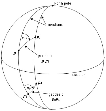
Figure 5.5 — Geodetic azimuths a12 from p1 to p2 and a34 from p3 to p4
5.8.3.5 Convergence of the meridian
Given a point ![]() in
the interior of the MP domain of a map projection, the meridian through that
point is projected to a curve in coordinate-space that passes through the
corresponding coordinate. The angle g at the coordinate in the clockwise direction from the curve to the v-axis (map-north)
direction shall be called the convergence of the meridian (COM) (see Figure 5.6).
in
the interior of the MP domain of a map projection, the meridian through that
point is projected to a curve in coordinate-space that passes through the
corresponding coordinate. The angle g at the coordinate in the clockwise direction from the curve to the v-axis (map-north)
direction shall be called the convergence of the meridian (COM) (see Figure 5.6).
The relationship  is
used to derive the formulae for COM from the mapping equations of each of the
map projections18. The COM angle is adjusted to the range
is
used to derive the formulae for COM from the mapping equations of each of the
map projections18. The COM angle is adjusted to the range![]() .
.
NOTE If
the map projection is conformal, then an equivalent relationship is given by: ![]() .
.
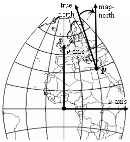
Figure 5.6 — Convergence of the meridian
EXAMPLE If p2 is directly map-north of p1 (it has a larger v coordinate-component), then the map azimuth is zero, but the geodetic azimuth may not be zero. The geodetic azimuth is approximately the sum of the map azimuth and the COM if the points are sufficiently close together.
5.8.4 Relationship to projection functions
5.8.4.1 Projection functions
Projection functions are defined in A.9. In some cases, the generating projection of a map projection CS is derived from a projection function. The derivation involves two steps. The first step is to restrict the domain of the projection function to a specified region of a given oblate ellipsoid so that the restricted function is one-to-one. The range of a projection function is a surface in 3D position-space. The second step is to associate that surface to 2D coordinate-space without introducing additional distortions.
In the case of planar projection functions, including the orthographic, perspective, and stereographic projection functions, the range is in a plane that can be identified with 2D coordinate-space by selecting an origin and unit axis points.
In the case of the cylindrical and conic projection functions, the range surface is a cylinder or a cone, respectively. These surfaces are developable surfaces and, except for a line of discontinuity, are homeomorphic to a subset of 2D coordinate-space with a homeomorphism that has a Jacobian determinant equal to one. Conceptually, these surfaces can be unwrapped to a flat plane without stretching the surface.
The polar stereographic MP (Table 5.22) is derived from the stereographic projection function, and in the spherical case, it is a conformal map projection. The same derivation may be applied to an oblate ellipsoid. However, the resulting map projection will not have the conformal property. For this reason, the generalization of the polar stereographic map projection mapping equations from the spherical case to the non-spherical oblate ellipsoid case is not derived from the polar stereographic projection function. Instead it is derived analytically to preserve the conformal property. Similarly, the Mercator map projection (Table 5.18) is designed to have the conformal property and is not derived from the cylindrical projection function even in the case of a sphere.
EXAMPLE Polar stereographic: Given a sphere with a polar point p, the tangent plane to the sphere at p and the opposite polar point v specify a stereographic planar projection function F (see A.9.2.3). The restriction of F to a subsurface of the sphere that excludes v, is the generating projection for the sphere case of a polar stereographic map projection. In Figure 5.7 the position s on the sphere is projected to point t on a plane.
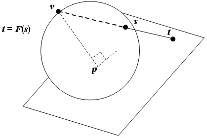
Figure 5.7 — Polar stereographic map projection
5.8.4.2 Map projection classification
The use of projection functions to derive map projections with desirable properties is limited, but does motivate some classifications of map projections. These classifications include tangent and secant map projections as well as conic and cylindrical map projections [SNYD, p. 5].
5.8.4.3 Cylindrical map projections
A map projection is classified as cylindrical if:
a) all meridians of the oblate ellipsoid project to parallel straight lines that are equally-spaced with respect to the longitude of the meridians, and
b) all parallels of the oblate ellipsoid project to parallel straight lines that are perpendicular to the meridian images.
As a consequence, ![]() for a cylindrical map projection.
for a cylindrical map projection.
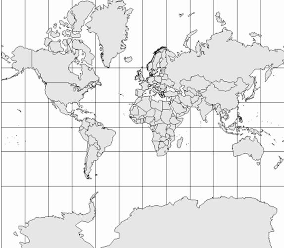
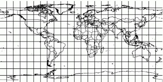
EXAMPLE The Mercator map projection (Table 5.18) and the equidistant cylindrical map projection (Table 5.23) are both classified as cylindrical map projections.
A cylindrical map projection is tangent if the longitudinal point distortion is equal to one along the equator. It is secant if the longitudinal point distortion is equal to one along two parallels equally-spaced from the equator in latitude. In that case, the parallel with positive latitude shall be called the standard parallel. Tangent and secant cylindrical map projections are illustrated in Figure 5.8.
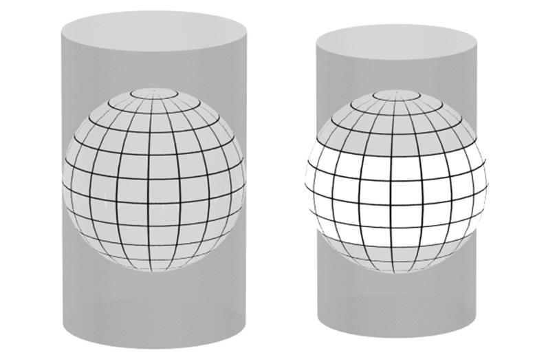
Figure 5.8 — Tangent and secant cylindrical map projections
5.8.4.4 Conic map projections
A map projection is classified as conic if:
a) all meridians of the oblate ellipsoid project to radial straight lines that are equally-spaced in radial angle with respect to the longitude of the meridians, and
b) all parallels of the oblate ellipsoid project to concentric arcs that are perpendicular to the meridian images.
As a consequence, g depends on l only for conic map projections because the projections of meridians are straight line segments with an angle depending only on the longitude.
EXAMPLE Lambert conformal conic (see Table 5.21) is classified as a conic projection.
A conic map projection is tangent if along one parallel the longitudinal point distortion is equal to one. It is secant if the longitudinal point distortion is equal to one along two parallels that are not symmetric about the equator. In that case, the two parallels shall be called the standard parallels (see Figure 5.9).
Figure 5.9 — Tangent and secant conical map projections
5.8.5 Map projection CS common parameters
To avoid negative coordinate-component values or to reduce the
magnitude of the values in a region of interest in the coordinate-space of a
map projection, two mapping equation parameters shall be provided to control
the position of the coordinate-space origin![]() . One, denoted as uF, shall be called the false easting and shall offset easting values. The second, denoted as vF, shall be called the false northing and shall offset northing values.
. One, denoted as uF, shall be called the false easting and shall offset easting values. The second, denoted as vF, shall be called the false northing and shall offset northing values.
A map projection CS specification may specify additional mapping equation parameters. The mapping equations parameters, including false easting and false northing shall be also be called the CS parameters.
The CS parameters longitude of origin, denoted by ![]() and
latitude of
origin, denoted by
and
latitude of
origin, denoted by ![]() are
historically associated with some map projection CSs. Typically, the position
with map coordinate
are
historically associated with some map projection CSs. Typically, the position
with map coordinate ![]() has
geodetic longitude equal to
has
geodetic longitude equal to![]() and/or
geodetic latitude equal to
and/or
geodetic latitude equal to![]() .
.
If ![]() is present
as a CS parameter in a map projection CS specification, it is used as the
longitudinal centring function parameter (see
is present
as a CS parameter in a map projection CS specification, it is used as the
longitudinal centring function parameter (see ![]() in Table 5.6.)
in Table 5.6.)
The CS parameter central scale, denoted by ![]() when
present, is intended to control the tangent/secant characteristics of the map
projection CS and is therefore close to, but does not generally exceed, 1,0. In
the case of a sphere,
when
present, is intended to control the tangent/secant characteristics of the map
projection CS and is therefore close to, but does not generally exceed, 1,0. In
the case of a sphere, ![]() corresponds
to a tangent projection, and
corresponds
to a tangent projection, and ![]() corresponds
to a secant projection. Typically, some point in the MP domain with geodetic
longitude equal to
corresponds
to a secant projection. Typically, some point in the MP domain with geodetic
longitude equal to ![]() and/or
geodetic latitude equal to
and/or
geodetic latitude equal to ![]() will
have a longitudinal point distortion equal to
will
have a longitudinal point distortion equal to![]() .
.
For some MP cases, if ![]() ,
there will exist a parallel with longitudinal point distortion equal to 1 at
each point on the parallel. The latitude of such a parallel is termed a secant latitude, or a latitude of true scale.
,
there will exist a parallel with longitudinal point distortion equal to 1 at
each point on the parallel. The latitude of such a parallel is termed a secant latitude, or a latitude of true scale.
NOTE Central
scale should not be confused with Map scale. Map scales (see 5.8.3.3) are typically much smaller in magnitude and are
applied directly to the coordinate-space. In particular, if a transverse Mercator map projection with
central scale value k0 = 0,9996 is to be scaled
50 000:1 on a map sheet display, then the mapping equations ![]() are evaluated with k0 = 0,9996 and the display coordinates
are evaluated with k0 = 0,9996 and the display coordinates ![]() are plotted on the
map sheet with s = (1/50 000).
are plotted on the
map sheet with s = (1/50 000).
5.8.6 Augmented map projections
5.8.6.1 Augmentation with ellipsoidal height
A 3D CS can be specified from a map projection CS. The canonical
embedding of a point (u, v) in R2 to
the point (u, v, 0) in the uv-plane of R3 allows map points in 2D
coordinate-space to be augmented with a third coordinate axis, the w-axis of R3. To be considered as a 3D CS,
an augmented 3-tuple (u, v, w) of coordinates in the augmented map projection coordinate-space shall be associated to a unique position in
position-space. The association is to ellipsoidal height![]() . Given an augmented
coordinate-tuple (u, v, w) for which (u, v) belongs to the coordinate range of the underlying generating
projection, the associated position is given in 3D geodetic coordinates (l, f, h) where (l, f,) is projected to (u, v) by the map projection mapping equations. The third
coordinate-space coordinate w is the vertical coordinate and the 3D geodetic coordinate
constraints on negative values of h impose corresponding constraints on
allowed values for w. In some application domains, other vertical coordinate measures
are used (see Clause 9).
Augmentation is restricted to ellipsoidal height in this International
Standard.
. Given an augmented
coordinate-tuple (u, v, w) for which (u, v) belongs to the coordinate range of the underlying generating
projection, the associated position is given in 3D geodetic coordinates (l, f, h) where (l, f,) is projected to (u, v) by the map projection mapping equations. The third
coordinate-space coordinate w is the vertical coordinate and the 3D geodetic coordinate
constraints on negative values of h impose corresponding constraints on
allowed values for w. In some application domains, other vertical coordinate measures
are used (see Clause 9).
Augmentation is restricted to ellipsoidal height in this International
Standard.
5.8.6.2 Distortion in augmented map projections
In addition to map projection distortion (see 5.8.3.1), augmentation causes additional distortion. Consider the two straight-line segments between the pairs of coordinate-space points {(u1, v1, 0), (u2, v2, 0)} and {(u1, v1, w), (u2, v2, w)} with w > 0 (see Figure 5.10). In augmented map projection geometry, the two line segments have the same length. The corresponding curve in position-space of the first line segment is a surface curve of the oblate ellipsoid (or sphere). The corresponding second curve is outside of the oblate ellipsoid (or sphere) and has longer arc length than the first, and the length difference increases with w.
In general, vertical angles are not preserved and the angular error will vary with the point distortion value. These and other distortions have profound implications for dynamic equations that are beyond the scope of this International Standard.
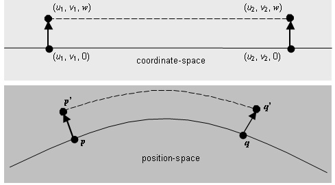
Figure 5.10 — Vertical distortion
5.9 CS specifications
5.9.1 Specification table elements and common functions and parameters
The CSs specified in this International Standard are presented in Table 5.8 through Table 5.35. Each CS specification specifies the values of all elements presented in Table 5.5.
Table 5.5 — Coordinate system specification elements
|
Element |
Definition |
|
Description |
A description of the CS including a common name, if any. |
|
CS label |
The label of the CS (see 13.2.2). |
|
CS code |
The code of the CS (see 13.2.3). |
|
Function type |
Either “generating function” or “map projection”. |
|
CS descriptor |
One of: 3D linear, 3D curvilinear, surface linear, surface curvilinear, map projection, 2D linear, 2D curvilinear, 1D linear, 1D curvilinear, or surface (map projection) and 3D (augmented map projection). |
|
Properties |
Either “none” or a list of one or more properties of the CS chosen from the following: orthogonal, not orthogonal, orthonormal, not orthonormal, conformal, or not conformal. Conformal and not conformal only apply to map projections. |
|
CS parameters and constraints |
The CS parameters (if any) along with any constraints on how those parameters interrelate, otherwise “none”. |
|
Coordinate-components |
Coordinate-component symbols and common names in a specified order. |
|
Domain of the generating function or mapping equations |
The domain of the CS generating function or the mapping equations. |
|
Generating function or mapping equations |
The CS generating function or mapping equations. |
|
Domain of the inverse of the generating function or mapping equations |
The domain of the inverse of the CS generating function or the domain of the inverse of mapping equations. |
|
Inverse of the generating function or mapping equations |
The inverse of the CS generating function or the inverse of mapping equations. |
|
COM |
For map projection CSs, the equation for g in radians. Otherwise "n/a". |
|
Point distortion |
For map projection CSs, the equation for k if conformal or |
|
Figures |
Zero or more figure(s) that explain and illustrate the CS. |
|
Notes |
Optional, non-normative information concerning the CS, otherwise "none". |
|
References |
The references (see 13.2.5). |
A specific ordering of coordinate-components for a coordinate n-tuple in a CS specification is required in this International Standard for clarity of presentation, to avoid ambiguity in the specification of the API, and, in the case of an orthonormal CS of CS type 3D, to insure the right-handed CS property (see 5.6.4). Alternatively, a coordinate-component value may be identified by its coordinate-component name and/or symbol in place of its identification by order in a coordinate-tuple.
Several specified CS generating functions and mapping equations and/or their inverses use some common intermediate functions or parameters associated with oblate ellipsoids. For clarity and concise presentation, these functions and parameters are defined in Table 5.6.
Table 5.6 — Common parameters and functions of an oblate ellipsoid
|
Function or parameter |
Symbol and defining expression |
|
major semi-axis |
|
|
minor semi-axis |
|
|
flattening |
|
|
(first) eccentricity |
|
|
second eccentricity |
|
|
radius of curvature in the prime vertical |
|
|
radius of curvature in the meridian |
|
|
meridional distance to equator |
|
|
longitudinal centring about |
|


NOTE 1 Replacing ![]() with
with ![]() gives the inverse of
the longitudinal centring function. That is:
gives the inverse of
the longitudinal centring function. That is:
![]()
NOTE 2 The function arctan2, used in many CS specification tables, is defined in A.8.2.
Table 5.7 presents a directory of the CS specifications in this International Standard. Each listed CS is specified in a separate table that is indicated by the hyperlink in the corresponding cell in the “Table number” column. Additional CSs may be added by registration (see Clause 13).
Table 5.7 — CS specification directory
|
Function
|
CS type |
Label and Description |
Table |
|
Generating function |
3D |
EUCLIDEAN_3D |
|
|
LOCOCENTRIC_EUCLIDEAN_3D |
|||
|
SPHERICAL |
|||
|
LOCOCENTRIC_SPHERICAL |
|||
|
AZIMUTHAL_SPHERICAL |
|||
|
LOCOCENTRIC_AZIMUTHAL_SPHERICAL |
|||
|
GEODETIC |
|||
|
PLANETODETIC |
|||
|
CYLINDRICAL |
|||
|
LOCOCENTRIC_CYLINDRICAL |
|||
|
Map projection |
Surface and augmented 3D |
MERCATOR |
|
|
OBLIQUE_MERCATOR_SPHERICAL |
|||
|
TRANSVERSE_MERCATOR |
|||
|
LAMBERT_CONFORMAL_CONIC |
|||
|
POLAR_STEREOGRAPHIC |
|||
|
EQUIDISTANT_CYLINDRICAL |
|||
|
Generating function |
Surface |
SURFACE_GEODETIC |
|
|
SURFACE_PLANETODETIC |
|||
|
LOCOCENTRIC_SURFACE_EUCLIDEAN |
|||
|
LOCOCENTRIC_SURFACE_AZIMUTHAL |
|||
|
LOCOCENTRIC_SURFACE_POLAR |
|||
|
2D |
EUCLIDEAN_2D |
||
|
LOCOCENTRIC_EUCLIDEAN_2D |
|||
|
AZIMUTHAL |
|||
|
LOCOCENTRIC_AZIMUTHAL |
|||
|
POLAR |
|||
|
LOCOCENTRIC_POLAR |
|||
|
1D |
EUCLIDEAN_1D |
5.9.2 Euclidean 3D CS specification
Table 5.8 — Euclidean 3D CS
|
Element |
Specification |
|
Description |
Euclidean 3D. |
|
Label |
EUCLIDEAN_3D |
|
Code |
1 |
|
Function type |
Generating function. |
|
CS descriptor |
3D linear. |
|
Properties |
Orthonormal. |
|
CS parameters and constraints |
none |
|
Coordinate-components |
u, v, w |
|
Domain of the generating function or mapping equations |
R3 |
|
Generating function or mapping equations |
|
|
Domain of the inverse of the generating function or mapping equations |
R3 |
|
Inverse of the generating function or mapping equations |
|
|
COM |
n/a |
|
Point distortion |
n/a |
|
Figures |
|
|
Notes |
Coordinate-space 3-tuples are identified with position-space 3-tuples. |
|
References |
[EDM] |


5.9.3 Lococentric Euclidean 3D CS specification
Table 5.9 — Lococentric Euclidean 3D CS
|
Element |
Specification |
|
Description |
Localized Euclidean 3D |
|
Label |
LOCOCENTRIC_EUCLIDEAN_3D |
|
Code |
2 |
|
Function type |
Generating function. |
|
CS descriptor |
3D linear. |
|
Properties |
Orthonormal. |
|
CS parameters and constraints |
Localization parameters: q: the lococentric origin in R3,
and Constraints: |
|
Coordinate-components |
u, v, w |
|
Domain of the generating function or mapping equations |
R3 |
|
Generating function or mapping equations |
|
|
Domain of the inverse of the generating function or mapping equations |
R3 |
|
Inverse of the generating function or mapping equations |
|
|
COM |
n/a |
|
Point distortion |
n/a |
|
Figures |
|
|
Notes |
1)
Euclidean 3D CS (see Table 5.8) is a special case with 2) The generating function is the composition of the generating function for Euclidean 3D CS (see Table 5.8) with the 3D localization operator (see 5.7). |
|
References |


5.9.4 Spherical CS specification
Table 5.10 — Spherical CS
|
Element |
Specification |
|
Description |
Spherical. |
|
Label |
|
|
Code |
3 |
|
Function type |
Generating function. |
|
CS descriptor |
3D curvilinear. |
|
Properties |
Orthogonal. |
|
CS parameters and constraints |
none |
|
Coordinate-components |
l : longitude in radians, |
|
Domain of the generating function or mapping equations |
|
|
Generating function or mapping equations |
|
|
Domain of the inverse of the generating function or mapping equations |
|
|
Inverse of the generating function or mapping equations |
|
|
COM |
n/a |
|
Point distortion |
n/a |
|
Figures |
|
|
Notes |
The spherical CS is not intrinsically associated with any specific sphere. |
|
References |
[HCP] |


5.9.5 Lococentric spherical CS specification
Table 5.11 — Lococentric spherical CS
|
Element |
Specification |
|
Description |
Localized spherical |
|
Label |
|
|
Code |
4 |
|
Function type |
Generating function |
|
CS descriptor |
3D curvilinear |
|
Properties |
Orthogonal |
|
CS parameters and constraints |
Localization parameters: q: the lococentric origin in R3,
and Constraints: |
|
Coordinate-components |
l : longitude in radians, |
|
Domain of the generating function or mapping equations |
|
|
Generating function or mapping equations |
|
|
Domain of the inverse of the generating function or mapping equations |
|
|
Inverse of the generating function or mapping equations |
|
|
COM |
n/a |
|
Point distortion |
n/a |
|
Figures |
|
|
Notes |
The generating function is the composition of the generating function for spherical CS (see Table 5.10) with the 3D localization operator (see 5.7). |
|
References |
[EDM] |


5.9.6 Azimuthal spherical CS specification
Table 5.12 — Azimuthal spherical CS
|
Element |
Specification |
|
Description |
Azimuthal spherical. |
|
Label |
|
|
Code |
5 |
|
Function type |
Generating function. |
|
CS descriptor |
3D curvilinear. |
|
Properties |
Orthogonal. |
|
CS parameters and constraints |
none |
|
Coordinate-components |
a : azimuth in radians, |
|
Domain of the generating function or mapping equations |
|
|
Generating function or mapping equations |
|
|
Domain of the inverse of the generating function or mapping equations |
|
|
Inverse of the generating function or mapping equations |
|
|
COM |
n/a |
|
Point distortion |
n/a |
|
Figures |
|
|
Notes |
none |
|
References |
[EDM] |


5.9.7 Lococentric azimuthal spherical CS specification
Table 5.13 — Lococentric azimuthal spherical CS
|
Element |
Specification |
|
Description |
Localized azimuthal spherical. |
|
Label |
|
|
Code |
6 |
|
Function type |
Generating function. |
|
CS descriptor |
3D curvilinear. |
|
Properties |
Orthogonal. |
|
CS parameters and constraints |
Localization parameters: q: the lococentric origin in R3,
and Constraints: |
|
Coordinate-components |
a : azimuth in radians, |
|
Domain of the generating function or mapping equations |
|
|
Generating function or mapping equations |
|
|
Domain of the inverse of the generating function or mapping equations |
|
|
Inverse of the generating function or mapping equations |
|
|
COM |
n/a |
|
Point distortion |
n/a |
|
Figures |
|
|
Notes |
The generating function is the composition of the generating function for azimuthal spherical (see Table 5.12) with the 3D localization operator (see 5.7). |
|
References |
[EDM] |


5.9.8 Geodetic 3D CS specification
Table 5.14 — Geodetic 3D CS
|
Element |
Specification |
|
Description |
Geodetic 3D. |
|
Label |
|
|
Code |
7 |
|
Function type |
Generating function. |
|
CS descriptor |
3D curvilinear. |
|
Properties |
Orthogonal. |
|
CS parameters and constraints |
a: major semi-axis length Constraints: |
|
Coordinate-components |
l : longitude in radians, |
|
Domain of the generating function or mapping equations |
|
|
Generating function or mapping equations |
|
|
Domain of the inverse of the generating function or mapping equations |
|
|
Inverse of the generating function or mapping equations |
|
|
COM |
n/a |
|
Point distortion |
n/a |
|
Figures |
|
|
Notes |
1) The surface geodetic CS (Table 5.24) is induced on the 3rd coordinate-component surface at any point for which h = 0. 2) If a = b, the geodetic latitude f coincides with the spherical latitude q (see Table 5.10). 3) The inverse generating function is not continuous on the oblate spheroid rotational axis. |
|
References |
[HEIK] |


5.9.9 Planetodetic 3D specification
|
Element |
Specification |
|
Description |
Planetodetic 3D. Geodetic 3D with longitude in opposite direction. |
|
Label |
|
|
Code |
8 |
|
Function type |
Generating function. |
|
CS descriptor |
3D curvilinear. |
|
Properties |
Orthogonal. |
|
CS parameters and constraints |
a: major semi-axis length Constraints: |
|
Coordinate-components |
f : geodetic latitude in
radians, |
|
Domain of the generating function or mapping equations |
|
|
Generating function or mapping equations |
|
|
Domain of the inverse of the generating function or mapping equations |
|
|
Inverse of the generating function or mapping equations |
|
|
COM |
n/a |
|
Point distortion |
n/a |
|
Figures |
|
|
Notes |
1) Similar to the geodetic 3D CS (see Table 5.14) except that longitude increases in the opposite direction. In particular, points on a planet surface rotating (prograde) into view have larger planetodetic longitudes than those points rotating out of view. This CS is also called planetocentric when a = b and planetographic when a > b. 2) The inverse generating function is not continuous on the oblate spheroid rotational axis. 3) The coordinate-component ordering differs from that of geodetic 3D CS to satisfy the right handedness requirement. |
|
References |
[RIIC] |


5.9.10 Cylindrical CS specification
Table 5.16 — Cylindrical CS
|
Element |
Specification |
|
Description |
Cylindrical. |
|
Label |
|
|
Code |
9 |
|
Function type |
Generating function. |
|
CS descriptor |
3D curvilinear. |
|
Properties |
Orthogonal. |
|
CS parameters and constraints |
none |
|
Coordinate-components |
|
|
Domain of the generating function or mapping equations |
|
|
Generating function or mapping equations |
|
|
Domain of the inverse of the generating function or mapping equations |
|
|
Inverse of the generating function or mapping equations |
|
|
COM |
n/a |
|
Point distortion |
n/a |
|
Figures |
|
|
Notes |
none |
|
References |
[EDM] |


5.9.11 Lococentric cylindrical CS specification
Table 5.17 — Lococentric cylindrical CS
|
Element |
Specification |
|
Description |
Localized cylindrical. |
|
Label |
|
|
Code |
10 |
|
Function type |
Generating function. |
|
CS descriptor |
3D curvilinear. |
|
Properties |
Orthogonal. |
|
CS parameters and constraints |
Localization parameters: q: the lococentric origin in R3,
and Constraints: |
|
Coordinate-components |
|
|
Domain of the generating function or mapping equations |
|
|
Generating function or mapping equations |
|
|
Domain of the inverse of the generating function or mapping equations |
|
|
Inverse of the generating function or mapping equations |
|
|
COM |
n/a |
|
Point distortion |
n/a |
|
Figures |
See Table 5.16. |
|
Notes |
1) The generating function is the composition of the cylindrical generating function (see Table 5.16) with 3D localization operator (see 5.7). 2) The domain of the inverse of the generating function is the set of all points not on the axis of the cylinder. |
|
References |
[EDM] |


5.9.12 Mercator CS specification
Table 5.18 — Mercator CS
|
Element |
Specification |
|
Description |
Mercator and augmented Mercator map projection coordinate systems. |
|
Label |
|
|
Code |
11 |
|
Function type |
Mapping equations. |
|
CS descriptor |
Surface (map projection) and 3D (augmented map projection). |
|
Properties |
Orthogonal, conformal. |
|
CS parameters and constraints |
|
|
Coordinate-components |
u: easting, and Augmented coordinate: |
|
Domain of the generating function or mapping equations |
|
|
Generating function or mapping equations |
|
|
Domain of the inverse of the generating function or mapping equations |
|
|
Inverse of the generating function or mapping equations |
For f, functional iteration is used for the representation of the inverse mapping equation [SNYD]. Superscripts involving i indicate elements in the iteration sequence.
|
|
COM |
|
|
Point distortion |
|
|
Figures |
Example Mercator map projection |
|
Notes |
1) Meridians project as straight lines that satisfy equations of the form u = a constant. Equally-spaced meridians project to evenly-spaced straight lines orthogonal to the u-axis. Parallels project to straight lines orthogonal to the projected meridians and satisfy equations of the form v = a constant. Evenly-spaced parallels project to unevenly-spaced parallel lines on the projection. The spacing of these lines increases with distance from the u-axis. 2) The meridian at 3) The point distortion equals 4) An alternate CS parameter set is given by: |
|
References |
[SNYD] |


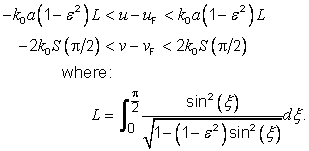
5.9.13 Oblique Mercator spherical CS specification
Table 5.19 — Oblique Mercator spherical CS
|
Element |
Specification |
|
Description |
Oblique Mercator and augmented oblique Mercator map projections of a sphere. |
|
Label |
OBLIQUE_MERCATOR_SPHERICAL |
|
Code |
12 |
|
Function type |
Mapping equations. |
|
CS descriptor |
Surface (map projection) and 3D (augmented map projection). |
|
Properties |
Orthogonal, conformal. |
|
CS parameters and constraints |
|
|
Coordinate-components |
u: easting, and Augmented coordinate: |
|
Domain of the generating function or mapping equations |
|
|
Generating function or mapping equations |
|
|
Domain of the inverse of the generating function or mapping equations |
|
|
Inverse of the generating function or mapping equations |
|
|
COM |
|
|
Point distortion |
|
|
Figures |
Example oblique Mercator spherical map projection |
|
Notes |
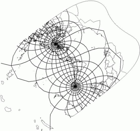
1) The method for specifying the central line by specifying two points on the central line can be accomplished by alternative formulations. The formulations for two such alternatives are provided below. Alternative a) In this
alternative the user specifies The CS parameter constraints are:
Alternative b) In this
alternative, a point (l1, f1) on the central line, a central
line crossing angle a1 at the point, and k0 at the point are specified. The central line crossing angle is
the angle between the central line and the parallel through the given point.
The positive sense of the angle is counter-clockwise from east. In this case
the origin The CS parameter constraints are:
The mathematical formulation is,
2) Point distortion is equal to k0 at all points on the central line. |
|
References |
[SNYD] |


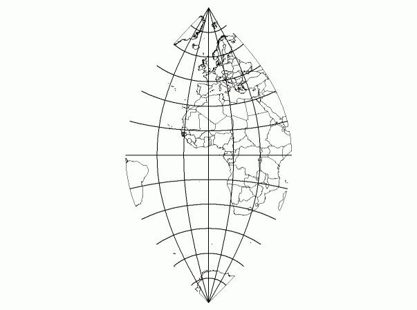
5.9.14 Transverse Mercator CS specification
Table 5.20 — Transverse Mercator CS
|
Element |
Specification |
|
Description |
Transverse Mercator and augmented transverse Mercator map projections. |
|
Label |
|
|
Code |
13 |
|
Function type |
Mapping equations. |
|
CS descriptor |
Surface (map projection) and 3D (augmented map projection). |
|
Properties |
Orthogonal, conformal. |
|
CS parameters and constraints |
|
|
Coordinate-components |
u:
easting, and Augmented coordinate: |
|
Domain of the generating function or mapping equations |
|
|
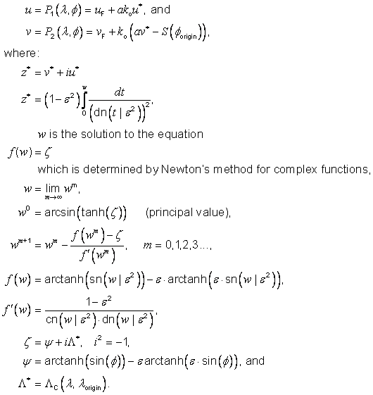
Generating function or mapping equations |
|
|
Domain of the inverse of the generating function or mapping equations |
|
|
Inverse of the generating function or mapping equations |
|
|
COM |
|
|
Point distortion |
|
|
Figures |
Example transverse Mercator map projection |
|
Notes |
1) As noted in [SNYD] and [LLEE], an iterative exact solution for the transverse Mercator forward and inverse conversions were developed by Prof. E. H. Thompson in 1945 and were formally published by L. P. Lee in 1962 [LLEE] with the permission of Professor Thompson. In 1980, J. Dozier published a report that adapted Lee’s results to a computerized solution, including complete program listings in the C language [DOZI]. The formulation used here is further adapted by Craig Rollins of the United States National Geospatial-Intelligence Agency (NGA) to include a central scale factor, a non-zero latitude origin and false easting and false northing offsets for both the easting and northing coordinate-components. 2) The complex functions sn(w |e2), cn(w |e2) and dn(w |e2) are defined in A.8.2. 3) The CS Generation function is extended by continuity to include the oblate ellipsoid pole points. 4) The domain of the inverse mapping equations covers the main region of interest. This domain can be extended to a larger region whose exact specification is complicated to define. 5) The iterative procedures used in both the forward and inverse formulations may be numerically ill conditioned near certain points. This occurs near the boundaries of the domains involved and near the equator for points with negative u values. When implementing these methods in software, special numerical methods may be required in the neighbourhood of such exceptional points. In particular, in the forward conversion, the exceptional points on the equator are avoided by restricting the procedure to use |l*| and then setting u to be negative when l*< 0. 6) The point distortion equals |
|
References |


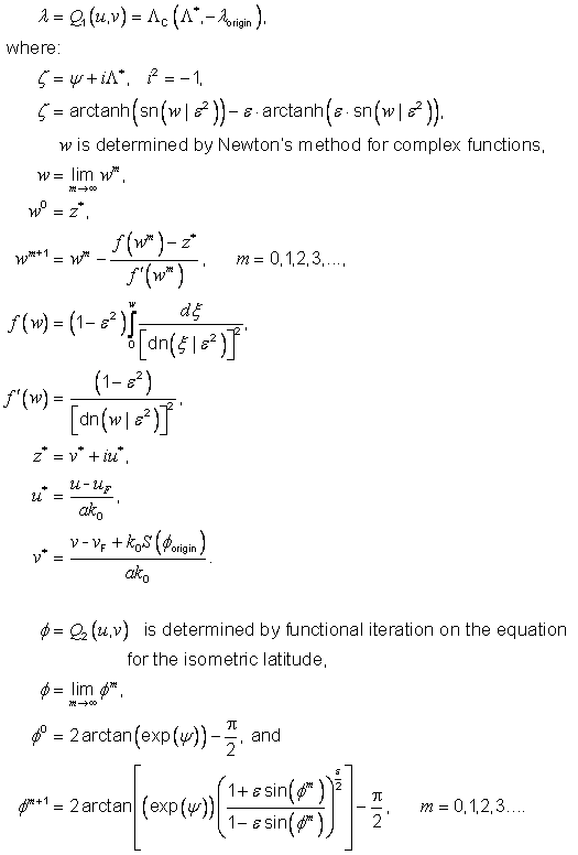


5.9.15 Lambert conformal conic CS specification
Table 5.21 — Lambert conformal conic CS
|
Element |
Specification |
|
Description |
Lambert conformal conic and augmented Lambert conformal conic map projections. |
|
Label |
|
|
Code |
14 |
|
Function type |
Mapping equations. |
|
CS descriptor |
Surface (map projection) and 3D (augmented map projection). |
|
Properties |
Orthogonal, conformal. |
|
CS parameters and constraints |
|
|
Coordinate-components |
u:
easting, and Augmented coordinate: |
|
Domain of the generating function or mapping equations |
|
|
Generating function or mapping equations |
|
|
Domain of the inverse of the generating function or mapping equations |
|
|
Inverse of the generating function or mapping equations |
|
|
COM |
|
|
Point distortion |
|
|
Figures |
Example Lambert conformal conic map projection |
|
Notes |
1)
2) The surface geodetic coordinate 3) The point distortion is unity along the standard parallel(s) f1 and f2. 4) An alternate CS parameter set is given by: |
|
References |
[SNYD] |


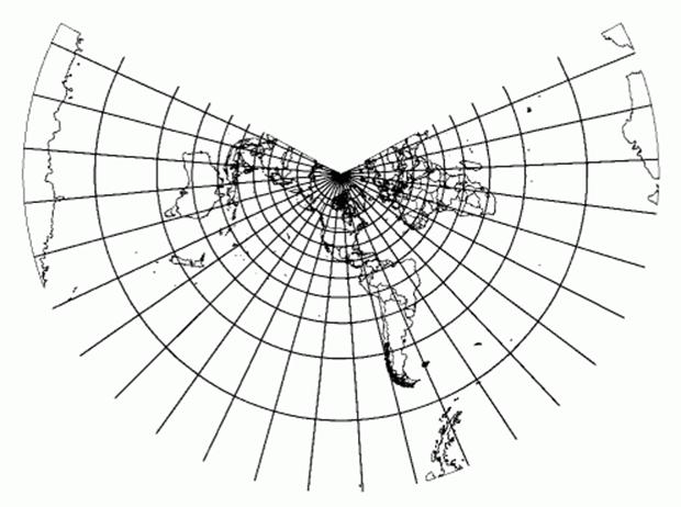

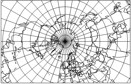
5.9.16 Polar stereographic CS specification
Table 5.22 — Polar stereographic CS
|
Element |
Specification |
|
Description |
Polar stereographic and augmented polar stereographic map projections. |
|
Label |
|
|
Code |
15 |
|
Function type |
Mapping equations. |
|
CS descriptor |
Surface (map projection) and 3D (augmented map projection). |
|
Properties |
Orthogonal, conformal. |
|
CS parameters and constraints |
|
|
Coordinate-components |
u: easting, and Augmented coordinate: |
|
Domain of the generating function or mapping equations |
|
|
Generating function or mapping equations |
|
|
Domain of the inverse of the generating function or mapping equations |
|
|
Inverse of the generating function or mapping equations |
For f, functional iteration is used for the representation of the inverse mapping equation. Superscripts involving m indicate elements in the iteration sequence.
|
|
COM |
|
|
Point distortion |
|
|
Figures |
Example polar stereographic map projection See also Figure 5.7 |
|
Notes |
1) Meridians project as straight lines radiating from the point 2) The point distortion values at pole is: 3) An alternate CS parameter set is given by: 4) In the case of a sphere, the mapping equations are derived from the stereographic projection (see Figure 5.7). 5) The CS Generation function is extended by continuity to include the oblate ellipsoid pole points. |
|
References |
[SNYD] |


5.9.17 Equidistant cylindrical CS specification
Table 5.23 — Equidistant cylindrical CS
|
Element |
Specification |
|
Description |
Equidistant cylindrical and augmented equidistant cylindrical map projections. |
|
Label |
|
|
Code |
16 |
|
Function type |
Mapping equations. |
|
CS descriptor |
Surface (map projection) and 3D (augmented map projection). |
|
Properties |
Orthogonal, non-conformal. |
|
CS parameters and constraints |
|
|
Coordinate-components |
u: easting, and Augmented coordinate: |
|
Domain of the generating function or mapping equations |
|
|
Generating function or mapping equations |
|
|
Domain of the inverse of the generating function or mapping equations |
|
|
Inverse of the generating function or mapping equations |
|
|
COM |
|
|
Point distortion |
|
|
Figures |
Example equidistant cylindrical map projection |
|
Notes |
1) Meridians project as straight lines that satisfy equations of the form u = a constant. Equally-spaced meridians project to evenly-spaced straight lines orthogonal to the u-axis. Parallels project to straight lines orthogonal to the projected meridians and satisfy equations of the form v = (a constant). 2) 3) The radius R of the conceptual cylinder is R = a k0. 4) An alternate CS parameter set is given by: |
|
References |
[SNYD] |


5.9.18 Surface geodetic CS specification
Table 5.24 — Surface geodetic CS
|
Element |
Specification |
|
Description |
Surface geodetic. |
|
Label |
|
|
Code |
17 |
|
Function type |
Generating function. |
|
CS descriptor |
Surface curvilinear. |
|
Properties |
Orthogonal. |
|
CS parameters and constraints |
a: major semi-axis length Constraints: |
|
Coordinate-components |
l : longitude in radians, and |
|
Domain of the generating function or mapping equations |
|
|
Generating function or mapping equations |
|
|
Domain of the inverse of the generating function or mapping equations |
|
|
Inverse of the generating function or mapping equations |
|
|
COM |
n/a |
|
Point distortion |
n/a |
|
Figures |
|
|
Notes |
1) The CS surface is the oblate ellipsoid (or sphere) surface excluding the pole points. 2) The geodetic 3D CS (Table 5.14) induces this CS on the 3rd coordinate-component surface at any point for which h = 0. 3) If a = b, the geodetic latitude f coincides with the spherical latitude q (see Table 5.10). 4) The inverse generating function is not continuous at the pole
points |
|
References |
[HEIK] |


5.9.19 Surface planetodetic CS specification
Table 5.25 — Surface planetodetic CS
|
Element |
Specification |
|
Description |
Surface planetodetic. Surface geodetic with longitude in opposite direction. |
|
Label |
|
|
Code |
18 |
|
Function type |
Generating function. |
|
CS descriptor |
Surface curvilinear. |
|
Properties |
Orthogonal. |
|
CS parameters and constraints |
a: major semi-axis length Constraints: |
|
Coordinate-components |
f : geodetic latitude in
radians, and |
|
Domain of the generating function or mapping equations |
|
|
Generating function or mapping equations |
|
|
Domain of the inverse of the generating function or mapping equations |
|
|
Inverse of the generating function or mapping equations |
|
|
COM |
n/a |
|
Point distortion |
n/a |
|
Figures |
|
|
Notes |
1) Similar to surface geodetic CS (see Table 5.24) except that longitude is in the opposite direction. In particular, points on a planet surface rotating (prograde) into view have larger planetodetic longitudes than those points rotating out of view. 2)
The inverse generating function
is not continuous at the pole points 3) The coordinate-components are ordered for compatibility with planetodetic 3D CS (see Table 5.15) |
|
References |
[RIIC] |


5.9.20 Lococentric surface Euclidean CS specification
Table 5.26 — Lococentric surface Euclidean CS
|
Element |
Specification |
|
Description |
Localization of Euclidean 2D CS into plane surface in 3D position-space. |
|
Label |
|
|
Code |
19 |
|
Function type |
Generating function. |
|
CS descriptor |
Surface linear. |
|
Properties |
Orthonormal. |
|
CS parameters and constraints |
Localization parameters: q: the lococentric origin in R3,
and Constraints: |
|
Coordinate-components |
u, v |
|
Domain of the generating function or mapping equations |
R2 |
|
Generating function or mapping equations |
|
|
Domain of the inverse of the generating function or mapping equations |
|
|
Inverse of the generating function or mapping equations |
|
|
COM |
n/a |
|
Point distortion |
n/a |
|
Figures |
|
|
Notes |
1)
The CS surface is the plane
specified by: 2) The generating function is the composition of the generating function for Euclidean 2D (see Table 5.29) with the surface localization operator (see 5.7). |
|
References |
[EDM] |


5.9.21 Lococentric surface azimuthal CS specification
Table 5.27 — Lococentric surface azimuthal CS
|
Element |
Specification |
|
Description |
Localization of azimuthal CS into plane surface in 3D position-space. |
|
Label |
|
|
Code |
20 |
|
Function type |
Generating function. |
|
CS descriptor |
Surface curvilinear. |
|
Properties |
Orthogonal. |
|
CS parameters and constraints |
Localization parameters: q: the lococentric origin in R3,
and Constraints: |
|
Coordinate-components |
a : azimuth in radians, and |
|
Domain of the generating function or mapping equations |
|
|
Generating function or mapping equations |
|
|
Domain of the inverse of the generating function or mapping equations |
|
|
Inverse of the generating function or mapping equations |
|
|
COM |
n/a |
|
Point distortion |
n/a |
|
Figures |
|
|
Notes |
1) The CS surface is the plane specified by: 2) The generating function is the composition of the generating function for azimuthal CS (see Table 5.31) with the 3D localization operator (see 5.7). |
|
References |
[EDM] |


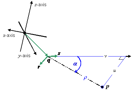
5.9.22 Lococentric surface polar CS specification
Table 5.28 — Lococentric surface polar CS
|
Element |
Specification |
|
Description |
Localization of polar CS into plane surface in 3D position-space. |
|
Label |
|
|
Code |
21 |
|
Function type |
Generating function. |
|
CS descriptor |
Surface curvilinear. |
|
Properties |
Orthogonal. |
|
CS parameters and constraints |
Localization parameters: q: the lococentric origin in R3,
and Constraints: |
|
Coordinate-components |
|
|
Domain of the generating function or mapping equations |
|
|
Generating function or mapping equations |
|
|
Domain of the inverse of the generating function or mapping equations |
|
|
Inverse of the generating function or mapping equations |
|
|
COM |
n/a |
|
Point distortion |
n/a |
|
Figures |
|
|
Notes |
1)
The CS surface is the plane
specified by: 2) The generating function is the composition of the generating function for polar CS (see Table 5.33) with the surface localization operator (see 5.7). |
|
References |
[EDM] |


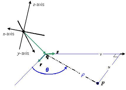
5.9.23 Euclidean 2D CS specification
Table 5.29 — Euclidean 2D CS
|
Element |
Specification |
|
Description |
Euclidean 2D. |
|
Label |
EUCLIDEAN_2D |
|
Code |
22 |
|
Function type |
Generating function. |
|
CS descriptor |
2D linear. |
|
Properties |
Orthonormal. |
|
CS parameters and constraints |
none |
|
Coordinate-components |
u, v |
|
Domain of the generating function or mapping equations |
R2 |
|
Generating function or mapping equations |
|
|
Domain of the inverse of the generating function or mapping equations |
R2 |
|
Inverse of the generating function or mapping equations |
|
|
COM |
n/a |
|
Point distortion |
n/a |
|
Figures |
|
|
Notes |
Coordinate-space 2-tuples are identified with position-space 2-tuples. |
|
References |
[EDM] |


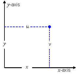
5.9.24 Lococentric Euclidean 2D CS specification
Table 5.30 — Lococentric Euclidean 2D CS
|
Element |
Specification |
|
Description |
Localized Euclidean 2D |
|
Label |
|
|
Code |
23 |
|
Function type |
Generating function. |
|
CS descriptor |
2D linear. |
|
Properties |
Orthonormal. |
|
CS parameters and constraints |
Localization parameters: q: the lococentric origin in R2,
and Constraints: |
|
Coordinate-components |
u, v |
|
Domain of the generating function or mapping equations |
R2 |
|
Generating function or mapping equations |
|
|
Domain of the inverse of the generating function or mapping equations |
R2 |
|
Inverse of the generating function or mapping equations |
|
|
COM |
n/a |
|
Point distortion |
n/a |
|
Figures |
|
|
Notes |
1) Euclidean 2D CS is a special case with 2) The generating function is the composition of the generating function for Euclidean 2D CS (see Table 5.29) with the 2D localization operator (see 5.7). |
|
References |
[EDM] |


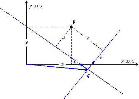
5.9.25 Azimuthal CS specification
Table 5.31 — Azimuthal CS
|
Element |
Specification |
|
Description |
Azimuthal coordinate system. |
|
Label |
|
|
Code |
24 |
|
Function type |
Generating function. |
|
CS descriptor |
2D curvilinear. |
|
Properties |
Orthogonal. |
|
CS parameters and constraints |
none |
|
Coordinate-components |
a : azimuth in radians, and |
|
Domain of the generating function or mapping equations |
|
|
Generating function or mapping equations |
|
|
Domain of the inverse of the generating function or mapping equations |
|
|
Inverse of the generating function or mapping equations |
|
|
COM |
n/a |
|
Point distortion |
n/a |
|
Figures |
|
|
Notes |
none |
|
References |
[EDM] |


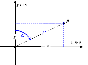
5.9.26 Lococentric azimuthal CS specification
Table 5.32 — Lococentric azimuthal CS
|
Element |
Specification |
|
Description |
Localization of azimuthal CS. |
|
Label |
|
|
Code |
25 |
|
Function type |
Generating function. |
|
CS descriptor |
2D curvilinear. |
|
Properties |
Orthogonal. |
|
CS parameters and constraints |
Localization parameters: q: the lococentric origin in R2,
and Constraints: |
|
Coordinate-components |
|
|
Domain of the generating function or mapping equations |
|
|
Generating function or mapping equations |
|
|
Domain of the inverse of the generating function or mapping equations |
|
|
Inverse of the generating function or mapping equations |
|
|
COM |
n/a |
|
Point distortion |
n/a |
|
Figures |
|
|
Notes |
The generating function is the composition of the generating function for azimuthal CS (see Table 5.31) with the 2D localization operator (see 5.7). |
|
References |
[EDM] |


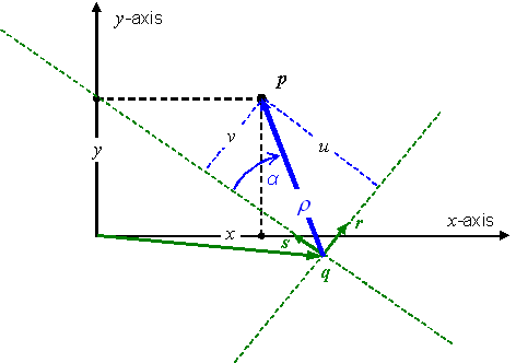
5.9.27 Polar CS specification
Table 5.33 — Polar CS
|
Element |
Specification |
|
Description |
Polar coordinate system. |
|
Label |
|
|
Code |
26 |
|
Function type |
Generating function. |
|
CS descriptor |
2D curvilinear. |
|
Properties |
Orthogonal. |
|
CS parameters and constraints |
none |
|
Coordinate-components |
|
|
Domain of the generating function or mapping equations |
|
|
Generating function or mapping equations |
|
|
Domain of the inverse of the generating function or mapping equations |
|
|
Inverse of the generating function or mapping equations |
|
|
COM |
n/a |
|
Point distortion |
n/a |
|
Figures |
|
|
Notes |
none |
|
References |
[EDM] |


5.9.28 Lococentric polar CS specification
Table 5.34 — Lococentric polar CS
|
Element |
Specification |
|
Description |
Localized polar. |
|
Label |
|
|
Code |
27 |
|
Function type |
Generating function. |
|
CS descriptor |
2D curvilinear. |
|
Properties |
Orthogonal. |
|
CS parameters and constraints |
Localization parameters: q: the lococentric origin in R2,
and Constraints: |
|
Coordinate-components |
|
|
Domain of the generating function or mapping equations |
|
|
Generating function or mapping equations |
|
|
Domain of the inverse of the generating function or mapping equations |
|
|
Inverse of the generating function or mapping equations |
|
|
COM |
n/a |
|
Point distortion |
n/a |
|
Figures |
|
|
Notes |
The generating function is the composition of the generating function for the polar CS (see Table 5.33) with the 2D localization operator (see 5.7). |
|
References |
[EDM] |


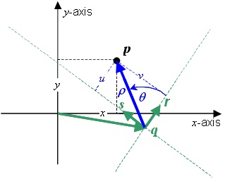
5.9.29 Euclidean 1D CS specification
Table 5.35 — Euclidean 1D CS
|
Element |
Specification |
|
Description |
Euclidean 1D. |
|
Label |
EUCLIDEAN_1D |
|
Code |
28 |
|
Function type |
Generating function. |
|
CS descriptor |
1D linear |
|
Properties |
none |
|
CS parameters and constraints |
none |
|
Coordinate-components |
u |
|
Domain of the generating function or mapping equations |
R1 |
|
Generating function or mapping equations |
|
|
Domain of the inverse of the generating function or mapping equations |
R1 |
|
Inverse of the generating function or mapping equations |
|
|
COM |
n/a |
|
Point distortion |
n/a |
|
Figures |
none |
|
Notes |
Coordinate-space 1-tuples are identified with position-space 1-tuples. |
|
References |
[EDM] |