[ Table of contents ]

10   SRF operations

10.1    Introduction

This International Standard specifies operations on SRF coordinates and, in the case of 3D object-spaces, on SRF spatial directions. Underlying these operations is the similarity transformation associated with two ORMs. Similarity transformations are treated first in 10.3. Then the general case of changing positional data from one SRF to another is specified in 10.4, followed by important special cases. The specification of a spatial direction in the context of an SRF is defined, and the general case of changing a SRF spatial direction to another SRF is specified (10.5).

Euclidean distance in 2D and 3D object-space is specified in 10.6. Distance and azimuth on the surface of an oblate ellipsoid (or sphere) are specified in 10.7. Vertical offset is defined in 9.3.

10.2    Notation and terminology

An important category of spatial operations is changing spatial information represented in one SRF to spatial information represented in a second SRF. For this category of operations, the adjective “source” shall be used to refer to the first SRF, and the adjective “target” shall be used to refer to the second SRF.

The notation in Table 10.1 is used throughout this clause.

Table 10.1 — Notation

 

10.3    Operations on ORMs

10.3.1    Introduction

The similarity transformations H_ST between source/target pairs ORM_S and ORM_T underlie the coordinate operations in 10.4. Given a set of n ORMs there are n(n-1) such source and target ORM pairs. Instead of specifying the full set of similarity transformations, this International Standard reduces the requirement to specifying the reference transformation H_SR from each object-fixed source ORM_S to the reference ORM_R for a given object. This subclause specifies the methods of expressing a similarity transformation H_ST in terms of the reference transformations for the source and target ORMs. The cases of ORMs for a single object are treated in 10.3.2. The more general cases in which ORM_S and ORM_T are ORMs for different objects are treated in 10.3.3.

10.3.2    ORMs for a single object

If ORM_S is an object-fixed ORM, its reference transformation H­_SR may be specified as a seven-parameter transformation in the 3D case (see 7.3.2) and a by four-parameter transformation in the 2D case (see 7.3.3). The general form of H­_SR in the 3D case is given by Equation (7). The form in the 2D case is similar. As vector operations, they are in the form of a scaled invertible matrix multiplication followed by a vector addition. This form of vector operation is an invertible affine transformation. In the 3D case using the notation of Equation (5):

NOTE          The processes by which ORMs for the Earth are established are based on physical measurements. These measurements are subject to error and therefore introduce various types of relative distortions between ORMs. Equation (7) is based on the assumption that positions in object-space are error free and the equation includes no compensation for these distortions.

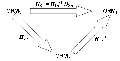
The reference transformation H_TR from ORM_T to ORM_R is similarly specified. An important operation is the similarity transformation H_ST from ORM_S to ORM_T, when neither the source nor the target is necessarily the reference ORM. The H_ST transformation may be expressed as the composition of  with  (the inverse of H_TR) as in Equation (8) (see Figure 10.1):

  Figure 10.1 — Composed transformations

The inverse operation  is also an affine transformation:

                   

Because the matrix  is a rotation matrix, its transpose  is also its inverse. Its inverse is also the matrix  corresponding to the reverse rotations of ORM_T with respect to ORM_R. In particular:

                   

and

                    .

The composite operation  reduces to:

where:

                   

 

If the rotation parameters are equal, then  is the identity matrix, and if, H_ST simplifies to a translation of the origin:

                    .

Equation (8) and Figure 10.1 also apply to the 2D case.

If the source ORM_S is a time-dependent ORM for a spatial object, ORM_S(t) shall denote the ORM_S at time t, and  shall denote the similarity transformation from the embedding of ORM_S(t) to the embedding of the object-fixed reference ORM_R. If the similarity transformation  can be determined, it is a time-dependent affine transformation. For a fixed value of time t₀, Equation (8) and Figure 10.1 generalize to . The generalizations to a time-dependent target ORM_T(t) are andfor the ORM_S static and time-dependent cases, respectively.

EXAMPLE            ORM_S(t) is the ORM EARTH_INERTIAL_J2000r0 at time t. ORM_R is the Earth reference ORM WGS_1984. Because ORM_S(t) and ORM_R share the same embedding origin, the  transformation is a (rotation) matrix multiplication operation (without vector addition). The matrix coefficients for selected values of t account for polar motion, Earth rotation, nutation, and precession. Predicted values for these coefficients are computed and updated weekly by the International Earth Rotation Service (IERS) [IERS] (see 7.5.2). See Annex B for other examples of dynamic ORM reference transformations.

10.3.3    Relating ORMs for different objects

If a spatial object S exists in the space of another spatial object T, and if ORM_R is the reference ORM for object T, and if the two objects are fixed with respect to each other, then H_SR shall denote a similarity transformation from the embedding of ORM_S to the embedding of ORM_R. H_SR is an affine transformation. If ORM_T is an object-fixed ORM for the object T then H_ST is given by Equation (8). The time dependent generalizations of Equation (8), defined in 10.3.2, are also applicable to this case.

EXAMPLE            ORM_S is an ORM for the space shuttle (as a spatial object). ORM­_R is the Earth reference ORM WGS_1984. When in orbit at time t, transforms positions with respect to ORM_S to positions with respect to ORM WGS_1984.

If the object-space of S and the object-space of T do not share locations or are otherwise unrelated, a similarity transformation between ORMs for the respective object-spaces is not defined. An abstract object S and a physical object T is an important instance of this case (see 10.4.6). However, if H_SR is an invertible affine transformation between ORM_S and the reference ORM for T, then, given an object-fixed ORM for object T, ORM_T, Equation (8) may be used to define an invertible affine transformation H_ST, from ORM_S to ORM_T.

10.4    Operations to change spatial coordinates between SRFs

10.4.1    Introduction

Given a coordinate in a source SRF, SRF_S, and a target SRF, SRF_T, the change coordinate SRF operation22 computes the corresponding coordinate  in SRF_T. The general case of changing the spatial coordinate of a location from SRF_S to SRF_T­ is presented in formulations in 10.4.2 for time-independent (static) and time-dependent ORM relationships. The general case assumes that the source coordinate corresponds to a location that exists in both the source and target object spaces.

In the general case, ORM_S and ORM_T may differ, and the coordinate systems, CS_S and CS_T, may differ. The formulation simplifies in the special case23 for which ORM_S = ORM_T or, more generally, in the case for which the associated normal embeddings match. This case is presented in 10.4.3. In a further specialization of the ORM_S = ORM_T case, it is assumed that CS_S and CS_T are geodetic and/or map projection CSs. These assumptions produce further simplifications (see 10.4.4).

The case for which CS_S = CS_T and ORM_S and ORM_T differ24 does not generally produce a computational simplification of the general case. However, when both the source and target SRFs are based on the CS LOCOCENTRIC_EUCLIDEAN_3D, a simplification is produced and is presented in 10.4.5. This case is important for change of direction operations (10.5.4).

An extension of the change SRF operation to the case of unrelated source and target object-spaces is presented in 10.4.6 for linear SRFs. In that case, the ORM transformation is only restricted to an invertible affine transformation.

10.4.2    Change coordinate SRF operation

SRF_S and SRF_T are two object-fixed SRFs for a spatial object and p is a point in object-space that is in the coordinate system domains for both SRFs. denotes the coordinate of p in SRF_S, and  denotes the coordinate of p in SRF_T. The determination of  as a function of  is an operation on the SRF pair (SRF_S, SRF_T). The most general form of the operation is:

where:

                   

See Figure 10.2. CS generating and inverse generation functions are specified in Clause 5.

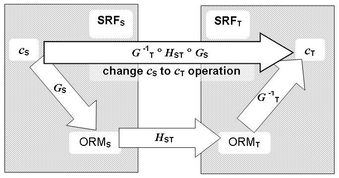
Figure 10.2 — Change coordinate SRF operation

Equation (10) is known as the Helmert transformation when H_ST is approximated with the Bursa-Wolfe equation (see Annex B).

In the time-dependent case, Equation (10) may be generalized to:

                    .

EXAMPLE 1         If SRF_S and SRF_T are two celestiodetic SRFs for the same spatial object with different ellipsoid RDs, Equation (10) transforms the coordinate  with respect to one oblate ellipsoid to  with respect to the other oblate ellipsoid.

NOTE          A transformation between two celestiodetic SRFs for the spatial object Earth is known as a horizontal datum shift. A number of numerical approximations developed to implement this operation have been published. Under the assumption of zero rotations and no scale differences (), a widely used approximation25 to directly transform  to , is the standard Molodensky transformation formula [83502T] as follows:

                   

where:

                   

The quantities  are defined in Table 5.6.

Equation (10) is only defined for a value of  in the CS_S domain if its corresponding position belongs to the CS_T range. If  is the domain of the inverse generating function  and  is the domain of the inverse generating function, Equation (10) is only defined for  in the set:

 

EXAMPLE 2         SRF_S is SRF GEOCENTRIC_WGS_1984 and SRF_T is an instance of SRFT MERCATOR, with ORM WGS_1984. Equation (10) is not defined for any that is on the z-axis of SRF_S, because the z-axis is not contained in the set in Equation (11).

SRF_T may optionally specify a valid-region  and may optionally specify an extended-valid region  (see 8.3.2.4). If  is the domain of the generating function, then . If Equation (10) is defined for,  may be valid, or extended valid  or neither. The set of  coordinates for which  is valid is:

             

where:

              .

In applications that functionally conform to an SRM profile, the domain of an SRF operation is restricted to the accuracy domain of the SRF as specified by that profile (see Clause 12).

10.4.3    The matched normal embeddings case

If both ORMs are the same²³ , or, more generally, if the corresponding parameters of the seven-parameter reference transformations of ORM_S and ORM_T match, is the identity transformation. Consequently, Equation (10) simplifies to:

EXAMPLE 1         If SRF_S is a celestiodetic SRF (see 8.4) and SRF_T is the celestiocentric SRF for the same ORM (ORM_S = ORM_T), then  is the identity and Equation (12) reduces to the geodetic generating function: .

EXAMPLE 2         If SRF_S is an induced surface celestiodetic SRF (see 8.4) and SRF_T is the 3D celestiodetic SRF for the same ORM (ORM_S = ORM_T), Equation (12) changes  from a coordinate of CS type surface to  a coordinate of CS type 3D.

If SRF_T is a 3D SRF that has ellipsoidal height designated as the vertical coordinate-component of the SRF (see 8.4), and SRF_S is the induced zero height surface SRF, the promotion operation converts a surface coordinate  in SRF_S to a 3D coordinate in SRF_T by setting the 1^st and 2^nd coordinate-components of  to the 1^st and 2^nd coordinate-components of  and setting the 3^rd coordinate-component, ellipsoidal height, to 0. Coordinate promotion is a special case of Equation (12). Applicable SRFs include those based on SRFT CELESTIODETIC, PLANETODETIC, and all map projection SRFTs

EXAMPLE 3         Reversing the roles of source and target SRFs in Example 2, if SRF_S is a celestiodetic 3D SRF and SRF_T is the (induced) surface celestiodetic SRF for the same ORM, Equation (12) is not defined for, unless. Equivalently, only coordinates of the form  belong to the set in Equation (11). Coordinates in SRF_S that are not on the oblate ellipsoid (or sphere) RD instance surface, can be projected to the surface along a coordinate curve by setting.

If SRF_S is a 3D SRF that has ellipsoidal height designated as the vertical coordinate-component of the SRF (see 8.4), and SRF_T is the induced zero height surface SRF, the truncation operation converts a 3D coordinate  in SRF_S to a surface coordinate , by setting the 1^st and 2^nd coordinate-components of  to the 1^st and 2^nd coordinate-components of. The point in object-space corresponding to  and the point in object-space corresponding to  are not the same point unless. Truncation, therefore, does not generally preserve location.

10.4.4    Map projection SRF and celestiodetic SRF with matched normal embeddings case

The CS generating function  for a map projection SRF (or, respectively, an augmented map projection SRF) is implicitly defined (see 5.8.2 or, respectively, 5.8.6) by the composition of the generating function for the surface geodetic CS (respectively, the geodetic 3D CS) with the inverse mapping equations  (respectively,) as:

                    .

If SRF_S and SRF_T are map projection SRFs for the same object, and the corresponding seven parameters of their reference transformations match, then Equation (12) becomes:

for:

             

Furthermore, if ORM_S = ORM_T, then  and Equation (13) simplifies to:

NOTE          If SRF_S is a map projection SRF, and SRF_T is the corresponding augmented map projection SRF based on the same ORM, then Equation (14) is equivalent to the promotion operation (see 10.4.3).

If SRF_T is a celestiodetic SRF and ORM_T = ORM_S, Equation (13) simplifies to:

                    .

Similarly, if SRF_S is a celestiodetic SRF and ORM_T = ORM_S, Equation (13) simplifies to:

                    .

10.4.5    Linear orthonormal 3D SRF to linear orthonormal 3D SRF cases

The special case of source and target SRFs based on the CS LOCOCENTRIC_EUCLIDEAN_3D is important for the treatment of directions (see 10.5). Every linear orthonormal CS may be viewed as an instance of a CS LOCOCENTRIC_EUCLIDEAN_3D. If SRF_S and SRF_T are two SRFT LOCOCENTRIC_EUCLIDEAN_3D based SRFs (see Table 8.11), then the SRF pair operation on  is determined by substituting the CS LOCOCENTRIC_EUCLIDEAN_3D (see Table 5.9) generating function  and its inverse  in Equation (10). If vectors  are the CS binding parameters for the SRFT LOCOCENTRIC_EUCLIDEAN_3D based SRF, may be expressed in the form of the affine transformation:

                   

where:

                   

The inverse generating function is expressed as:

                   

where:.

 

If vectors  are the CS binding parameters for SRF_S and SRF_T respectively (see Table 8.11), then substituting the expression in Equation (9) for H_ST, Equation (10) specializes to:

In the case that the corresponding seven parameters of the reference transformations of ORM_S and ORM_T match, Equation (12) specializes to Equation (16):

 

10.4.6    Changing abstract space linear SRF coordinates to a linear SRF in the space of another object

Engineering designs and other abstract models are often intended for realization in the physical world.

EXAMPLE            A building plan is designed in the source SRF_S, an abstract space LOCAL_SPACE_RECTANGULAR_3D SRF. A terrestrial site survey establishes the origin of the target SRT_T, a LOCAL_TANGENT_SPACE_EUCLIDEAN SRF. Source coordinates are identified to target coordinates by: where is a scale factor.

More generally, abstract models are scaled, rotated, or otherwise transformed by an invertible matrix W before a source coordinate is identified to a target coordinate. This identification may be viewed as a change coordinate SRF operation from  in SRF_S, an abstract space LOCAL_SPACE_RECTANGULAR_3D SRF, to a coordinate in SRF_T, a physical world LOCOCENTRIC_EUCLIDEAN_3D  SRF. In the notation of 10.4.5:

                   

Define an invertible affine transformation as (see 10.3.3). Substitute this in Equation (10) and simplify:

This illustrates that the identification  may be viewed as a change coordinate SRF operation.

NOTE       Equation (17) illustrates that digital graphic composite pattern modelling techniques such as SceneGraph trees that use scale and rotation matrices W together with translation operations at each tree node are special cases of Equation (10). See also 10.5.4 Example 2.

10.5    Spatial directions and change SRF operations on directions

10.5.1    Introduction

In 3D position-space, a direction is unambiguously specified by a normalized vector. The direction specified is translation independent. This is illustrated by lines through points in a given direction n (see A.7.1.1 Example 1). All such lines are parallel. This translation invariance carries over to the coordinate-space of a linear CS, but not to other CSs with vector space structure. In particular, an augmented map projection inherits the vector space structure of 3D Euclidean coordinate-space, but the “up pointing” vector n = (0, 0, 1) points in different spatial directions (in position-space) depending on the map coordinate location from which n is viewed.

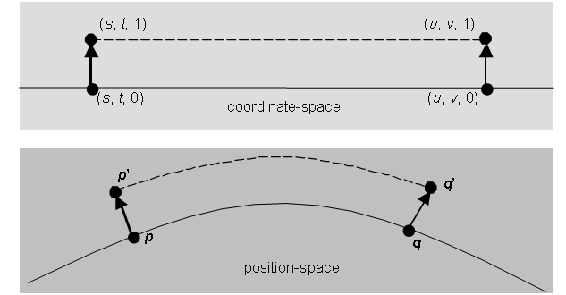
Figure 10.3 — Coordinate-space and position-space directions compared

In Figure 10.3, distinct position points p and q on the ellipsoid surface are projected to augmented map coordinates (s, t, 0) and (u, v, 0). Starting at these map coordinates, the coordinates one unit away in direction n are (s, t, 1) and (u, v, 1) respectively. In an augmented map projection, these coordinates correspond to the position-space points p’ and q’. The direction from p’ to p is not the same as the direction from q’ to q. It is noted in 5.8.6.2 that augmented map projections are not vertically conformal, therefore angular relationships of spatial directions are generally not preserved by augmented map projections.

A linear CS will not preserve angular relationships between directions unless the CS is also orthonormal. In an SRF based on a linear orthonormal CS, the translation invariant vector space structure of the abstract CS carries over to the spatial CS because the underlying normal embedding preserves angles and distances.

The coordinate-space of a curvilinear CS does not have a linear vector space structure so there is no natural way to specify a translation invariant direction with curvilinear coordinates. An SRF based on a curvilinear CS requires a uniform method associating a unique linear orthonormal CS based SRF to each coordinate in the interior of the CS domain. This association is defined in 10.5.2.

10.5.2    Specification of direction

In this International Standard, a direction in a 3D orthogonal26 SRF_S is expressed as a combination of a normalized vector and a reference coordinate. The normalized vector is in a 3D linear orthonormal SRF, denoted by SRF_L. If SRF_S is curvilinear, SRF_L is uniquely defined for each reference coordinate using the normalized tangent vectors to the coordinate-component curves at the reference coordinate. These vectors are used as SRF parameters for SRFT LOCOCENTRIC_EUCLIDEAN_3D with ORM_S to specify SRF_L. SRF_L is termed the local tangent frame at the reference coordinate.

The same definition is applicable if SRF_S is linear. In the linear case, SRF_L at reference coordinate (0, 0, 0) coincides with SRF_S as a spatial CS. Also in the linear case, the normalized vector representing the direction is independent of the reference coordinate used. The linear case includes SRFs that are based on SRFTs CELESTIOCENTRIC, LOCAL_TANGENT_SPACE_EUCLIDEAN, LOCOCENTRIC_EUCLIDEAN_3D, and LOCAL_SPACE_RECTANGULAR_3D.

Given a coordinate c = (u₀, v₀, w₀) in the interior of the domain of a 3D orthogonal SRF_S, the local tangent frame at coordinate c, SRF_L, is the SRF specified by the SRFT LOCOCENTRIC_EUCLIDEAN_3D with ORM_S and the following SRF parameters:

where:

             

 

The vectors r and s are termed the local tangent vectors at c. Coordinate-component curves are defined in 5.5.3.

NOTE 1       The tangent vector to the 3^rd coordinate-curve at (u₀, v₀, w₀) points in the same direction as the vector  because of the coordinate-component ordering restriction specified in 5.6.4.

A direction in an orthogonal CS based SRF_S shall be comprised of:

a)       a coordinate c in the interior of the CS domain of SRF_S, and

b)       a normalized vector n in the local tangent frame at c.

The coordinate c is termed the reference coordinate of the direction and its corresponding position is termed the reference position for the direction. The vector n is termed the direction vector at c.

NOTE 2       The local tangent frame at a coordinate is an instance of the SRFT LOCOCENTRIC_EUCLIDEAN_3D that provides a vector space setting for vector operations on direction vectors at c.

EXAMPLE 1         If SRF_S is a LOCOCENTRIC_EUCLIDEAN_3D SRF with SRF parameters q, r and s, and c is an SRF_S reference coordinate, then local tangent vectors at c are equal to the SRF parameters r and s. If c = (0,0,0), then SRF_L = SRF_S.

EXAMPLE 2         SRF_S is an EQUATORIAL_INERTIAL SRF. This SRF is based on the SPHERICAL CS. If  is a reference coordinate, then the local tangent vectors at c are:

EXAMPLE 3         SRF_S is a CELESTIODETIC SRF. This SRF is based on the GEODETIC CS. If  is a reference coordinate, then the local tangent vectors at c are:

The vector  

In this example, SRF_L is an LOCAL_TANGENT_SPACE_EUCLIDEAN SRF with SRF parameters .

EXAMPLE 4      SRF_S is based on a conformal map projection CS. If  is a reference coordinate, and  is the corresponding celestiodetic coordinate, then the local tangent vectors at c are:

In this example, SRF_L is an LOCAL_TANGENT_SPACE_EUCLIDEAN SRF with SRF parameters .

10.5.3    Changing the reference coordinate of a direction

Given a direction represented with direction vector n₁ at c₁, the same direction may be represented at another reference coordinate c₂ in the same SRF, with direction vector n₂. The direction vector n₂ is computed as:

 

The local tangent vectors are computed as in Equation (18). Equation (19) is derived from Equation (16) by dropping the translation term since directions are translation invariant.

If the SRF is based on a linear CS, then the matrix in Equation (19) is the identity matrix and n₁ = n₂. This implies that in an SRF based on a linear orthonormal CS, a direction vector is independent of the reference coordinate. Thus, Equation (19) is only of interest in the case of a curvilinear SRF.

10.5.4    Changing the SRF representation of a direction

Given a direction represented with direction vector n_S at c_S in SRF_S, the same direction may be represented at reference coordinate c_T, with direction vector n_T in SRF_T. If H_ST is the similarity transformation from ORM_S to ORM_T and T_ST is the matrix in the last term in Equation (15), then the direction vector n_T is computed as:

 

Equation (20), is derived from Equation (15) by dropping the translation term since directions are translation invariant and dropping the scale factor since n_T is a normalized vector.

EXAMPLE 1         SRF_S is SRF GEODETIC_WGS_1984 and SRF_T is SRF GEOCENTRIC_WGS_1984. With SRF_S reference coordinate , the Washington monument, an obelisk, points approximately in the direction  at c_S. In this example, ORM_S = ORM_T so that T_ST is the identity matrix, and because SRF_T is based on SRFT CELESTIOCENTRIC, is also the identity matrix. Consequently Equation (20) reduces to:

               

Then using the expression in 10.5.2 Example 3 for t:

               

So that the direction vector in SRF GEOCENTRIC_WGS_1984 is.

The case of changing an abstract space linear SRF direction vector n_S to a direction vector n_T in a linear SRF in the space of another object is based on Equation (17). In the notation of 10.4.6:

 

Since a direction vector is normalized, division by the determinant cancels any scaling by matrix W. R_S is a rotation matrix and therefore its determinant is 1.

EXAMPLE 2         In ISO/IEC FDIS 18023-1:2005, if an instance of the class <DRM Geometry Model Instance> has a component of class <DRM World Transformation>, that component specifies an invertible matrix W and a coordinate c in the <DRM Environment Root> SRF. If c_S and n_S are a reference coordinate and a direction vector in an associated LOCAL_SPACE_RECTANGULAR_3D <DRM Geometry Model>, and SRF_T is the local tangent frame at c, then Equation (17) and Equation (21) may be used to compute c_T and n_T, respectively. The methods of 10.4.3 may be used to further change c_T from SRF_T to the <DRM Environment Root> SRF. This procedure to change <DRM Geometry Model> coordinates and directions to the environment root SRF is termed "model instancing".

10.6    Euclidean distance

This International Standard supports an operation to return the Euclidean distance between two object-space locations using the coordinates of those locations in an SRF.

If c₁ and c₂ are two coordinates in an SRF, and if G is the generating function of the CS of the SRF, the Euclidean distance d_E between the corresponding points in object-space is given by:

             

where d is the Euclidean metric.

10.7    Geodesic distance and azimuth on an oblate ellipsoid

10.7.1    Introduction

This International Standard supports the geodesic distance and azimuth operations for SRFs that have ellipsoidal height designated as the vertical coordinate-component (see 8.4). These SRFs include those based on SRFT CELESTIODETIC, PLANETODETIC, and all map projection SRFTs.

The zero vertical coordinate-component surface for such an SRF is an oblate ellipsoid. Two distinct points on the surface of the oblate ellipsoid are connected by a surface curve called a geodesic as defined in A.7.3. The distance along the curve between the two points is called the geodesic distance. At each point, the angle between the geodesic and the meridian at the point as defined in 5.8.3.4 is the azimuth at the point with respect to the other point. The operations to return the geodesic distance and azimuths given the surface coordinates of the points are supported in the API.

10.7.2    Geodesic distance

For an oblate ellipsoid, a geodesic does not, in general, lie completely in any single plane [RAPP1] [RAPP2]. If ( λ₁, φ₁) and ( λ₂, φ₂) are the surface celestiodetic coordinates of two points lying on the oblate ellipsoid surface with parameters a and e, and, the geodesic distance  between the points [PEAR] is given by:

             

In the general case, two surface coordinates c₁ and c₂ are converted to celestiodetic coordinates using the operations defined in 10.4.4. In particular, in the case of a map projection SRF, if Q is inverse mapping equations for the SRF, then:

                   

NOTE          This is an elliptic integral and the development of approximation equations for has been the subject of much research. There are approximation formulas for the short distance case where  ≤ 200 km, for the medium distance case where  ≤ 1000 km and for the long lines case where the points are antipodal or near antipodal. Two points on the oblate ellipsoid are exactly antipodal when |(λ₂ - λ₁)| = π and φ₁ = -φ₂. There are also special cases when. A thorough exposition of geodesic distance approximations is given in [RAPP1] [RAPP2].

10.7.3    Geodetic azimuth

Geodetic azimuth is defined in 5.8.3.4. On a sphere, a geodesic between two points is an arc of a great circle and the problem of computing the angles of a spherical triangle can be solved in closed form. In the general case of an oblate ellipsoid, the problem of computing the angles of an elliptical triangle does not have a closed solution. Several different approximations are commonly used.

NOTE          Some algorithms are designed to compute both the geodesic distance and the azimuths associated with two points.

[ Table of contents ]